Numpy arrays
We are going to deal with numpy arrays along this practice session. Prior to implementing any formulas using Numpy, let’s be more knowledgeable with this data structure.
Importing needed librairies:
import os
import pandas as pd
import numpy as np
import matplotlib.pyplot as plt
A scalar
A real number, an element of a fied. Enables to define vector space.
scalar = 4.2 # a real number
A vector
Creation
We are going to use the array constructor to create such vector.
The numpy ndim attribute gives the number of dimensions.
The numpy shape attribute gives the number of elements in each dimensions, hence returning a tuple.
The numpy size attribute gives the number of elements in the array. You could also do the product between each number of elements in each dimension to get the same value: np.prod(array.shape).
vector_1D = np.array([4])
vector_1D_of_multiple_elements = np.array([1,2,3,4,5,6])

print(vector_1D, vector_1D_of_multiple_elements)
print(vector_1D.shape, vector_1D_of_multiple_elements.shape)
print(vector_1D.ndim, vector_1D_of_multiple_elements.ndim)

print(vector_1D.size, vector_1D_of_multiple_elements.size)
[4] [1 2 3 4 5 6]
(1,) (6,)
1 1
1 6
Transpose vector
You can use T attribute to transpose a vector or matrix.
For a 1D vector, the transpose does not change its representation.
But it is going to make sense as we express a vector as matrix column vector vs vector as matrix row vector.
(vector_1D_of_multiple_elements.T,
 vector_1D_of_multiple_elements.T.shape) # same thing (in terms of representation)
(array([1, 2, 3, 4, 5, 6]), (6,))
(vector_1D_of_multiple_elements,
vector_1D_of_multiple_elements.shape,
vector_1D_of_multiple_elements.ndim)
(array([1, 2, 3, 4, 5, 6]), (6,), 1)
A matrix
Creation
1st dimension can be seen as the “rows” dimension.
2nd dimension can be seen as the “columns” dimension.
Hence using the array constructor: the argument can be a list of lists, as stacking rows of p features (column elements).
matrix = np.array([
            [ 1, 2, 3],
            [ 4, 5, 6]
          ])
matrix, matrix.shape, matrix.ndim, matrix.size
(array([[1, 2, 3],
        [4, 5, 6]]),
 (2, 3),
 2,
 6)
transpose matrix
Transposing a matrix results in inversing the shape tuple.
In 2D matrix example: from 2 rows and 3 columns, we got 3 rows and 2 columns.
matrix.T, matrix.T.shape, matrix.T.ndim, matrix.size
(array([[1, 4],
        [2, 5],
        [3, 6]]),
 (3, 2),
 2,
 6)
Re-shape a vector or matrix
It is possible to give a new shape to an array without changing its data, this is enabled by the numpy reshape method.
A vector of one element.
vector_1D.size
1
A 2D matrix of 1 element (one row, one column):
vector_1D.reshape((1,1))
array([[4]])
A 3D matrix of 1 element (one row, one column, on “depth” (if we see it as a cube)):
vector_1D.reshape((1,1,1))
array([[[4]]])
Nor the number of elements neither the values did change.
vector_1D_of_multiple_elements.size
6
Same thing using the vector of 6 elements, turning into a matrix of 3 rows and 2 columns (still valid shape for the total number of elements):
vector_1D_of_multiple_elements.reshape(3,2)
array([[1, 2],
       [3, 4],
       [5, 6]])
Or a matrix of 2 rows and 3 columns:
vector_1D_of_multiple_elements.reshape(2, 3)
array([[1, 2, 3],
       [4, 5, 6]])
pd.DataFrame
Recall pandas library ? Sometimes it is easier to see a 2D numpy array as a DataFrame using its constructor.
For a 1D vector it is seen as a column:
pd.DataFrame(vector_1D_of_multiple_elements)
| 0 | |
|---|---|
| 0 | 1 |
| 1 | 2 |
| 2 | 3 |
| 3 | 4 |
| 4 | 5 |
| 5 | 6 |
For the 2D matrix:
pd.DataFrame(matrix)
| 0 | 1 | 2 | |
|---|---|---|---|
| 0 | 1 | 2 | 3 |
| 1 | 4 | 5 | 6 |
Transposing the vector of multiple elements didn’t change anything (as for its numpy array representation):
pd.DataFrame(vector_1D_of_multiple_elements.T)
| 0 | |
|---|---|
| 0 | 1 |
| 1 | 2 |
| 2 | 3 |
| 3 | 4 |
| 4 | 5 |
| 5 | 6 |
If we were to use the DataFrame constructor on the vector, and THEN use the attribute shape (recall that pandas also share similarities in its API with numpy one), you can see that the vector as been turn in a “(matrix) column vector” (a matrix with only one column and multiple rows).
pd.DataFrame(vector_1D_of_multiple_elements).shape
(6, 1)
Hence using T, you get a (matrix) row vector (matrix with multiple columns but only one row):
pd.DataFrame(vector_1D_of_multiple_elements).T
| 0 | 1 | 2 | 3 | 4 | 5 | |
|---|---|---|---|---|---|---|
| 0 | 1 | 2 | 3 | 4 | 5 | 6 |
Vector “as” matrix
In linear algebra, a column vector or column matrix is an m × 1 matrix, that is, a matrix consisting of a single column of m elements
as_matrix = vector_1D_of_multiple_elements.reshape(6, 1) # 6 rows, 1 column
pd.DataFrame(as_matrix)
| 0 | |
|---|---|
| 0 | 1 |
| 1 | 2 |
| 2 | 3 |
| 3 | 4 |
| 4 | 5 |
| 5 | 6 |
Similarly, a row vector or row matrix is a 1 × m matrix, that is, a matrix consisting of a single row of m elements.
as_matrix = vector_1D_of_multiple_elements.reshape(1, 6) # 1 column, 6 rows
pd.DataFrame(as_matrix)
| 0 | 1 | 2 | 3 | 4 | 5 | |
|---|---|---|---|---|---|---|
| 0 | 1 | 2 | 3 | 4 | 5 | 6 |
Operations between vectors and/or matrices
Dot Product (produit scalaire)
vector1 = np.array([1,2,3,4,5])
vector2 = np.array([2,4])
try:
    np.dot( vector1, vector2 )
except:
    print("Not the same number of elements to perform a dot product (must be aligned)")
Not the same number of elements to perform a dot product (must be aligned)
vector2 = np.array([2,4,1,1,1])
The algebraic dot product gives the sum of the component-wise multiplications from vector1 and vector2 (in Cartesian coordinates; in Euclidian ones you multiply the magnitude of each and the cosine of the angle between them, and of course the definitions here are equivalents as in cartesian coordinates each component of the vector can be seen as a magnitude that multiplies a corresponding unit vector in an orthogonal basis. Hence each vector can be expressed as the sum of those basis vectors with corresponding component. The geometric dot product resulting in a cosine: \(cos(\theta) = 1\)) for 2 components in the same \(e_i\) and \(cos(\theta) = 0\) for 2 components in different \(e_i\). Hence Algebraic dot product equals geometric dot product).
The algebraic dot product returns a scalar.
np.dot(vector1, vector2) # 1*2 + 2*4 + 3*1 + 4*1 + 5*1
22
try:
    np.dot(vector1.reshape(1,5), vector2.reshape(1,5))
except:
    print("Again, not aligned because in maths you do the transpose of the vector1 ")
Again, not aligned because in maths you do the transpose of the vector1

# this works
result_dot_product = np.dot(vector1.reshape(1,5), vector2.reshape(1,5).T)
# this works
result_matrix_product = np.matmul(vector1.reshape(1,5), vector2.reshape(1,5).T)
# same result
result_dot_product, result_matrix_product
(array([[22]]), array([[22]]))
“componentwise” multiplications (i.e. Hadamard Product on Matrices, or column/row vector)
Not to confuse with dot product:
vector1 * vector2 # vector of element multiplications
Returns a vector of the component-wise multiplications.
array([2, 8, 3, 4, 5])
# same result
np.multiply(vector1, vector2)
array([2, 8, 3, 4, 5])
np.multiply(vector1.reshape(1,5), vector2.reshape(1,5))
array([[2, 8, 3, 4, 5]])
Broadcasting rules numpy
Refers to how numpy treats arrays with different shapes during arithmetic operations.
Subject to certain constraints, the smaller array is “broadcast” across the larger array so that they have compatible shapes!
- Same shapes, no problem:
vector1 = np.array([1,2,3])
vector2 = np.array([1,2,3])

vector1 + vector2
array([2, 4, 6])
- different shapes, what to do ?
**Example1:**
vector1 = np.array([2])
vector2 = np.array([1,2,3])
vector1.shape, vector2.shape
((1,), (3,))
vector1 + vector2
array([3, 4, 5])
This is the same thing as:
vector1_transformed = np.tile(vector1, reps=(3,))
print( vector1_transformed )
vector1_transformed + vector2
[2 2 2]


array([[3, 4, 5]])
from CS231N Stanford:
- If the arrays do not have the same rank (number of dimensions), prepend the shape of the lower rank array with 1s until both shapes have the same length.
- The two arrays are said to be compatible in a dimension if they have the same size in the dimension, or if one of the arrays has size 1 in that dimension.
- The arrays can be broadcast together if they are compatible in all dimensions.
After broadcasting:
- After broadcasting, each array behaves as if it had shape equal to the elementwise maximum of shapes of the two input arrays.
- In any dimension where one array had size 1 and the other array had size greater than 1, the first array behaves as if it were copied along that dimension.
vector1 = np.array([[1]])
vector2 = np.array([1,2,3])
vector1.shape, vector2.shape
((1, 1), (3,))
prepending ones, the last dimension of the array will be “strecthed” so the number of elements match with the one of the first array
vector1 + vector2
array([[2, 3, 4]])
**Example2:**
vector1 = np.array([[1], [2]]) # 2 rows, 1 column
vector2 = np.array([1,2,3]) # 1D vector
vector1.shape, vector2.shape
((2, 1), (3,))
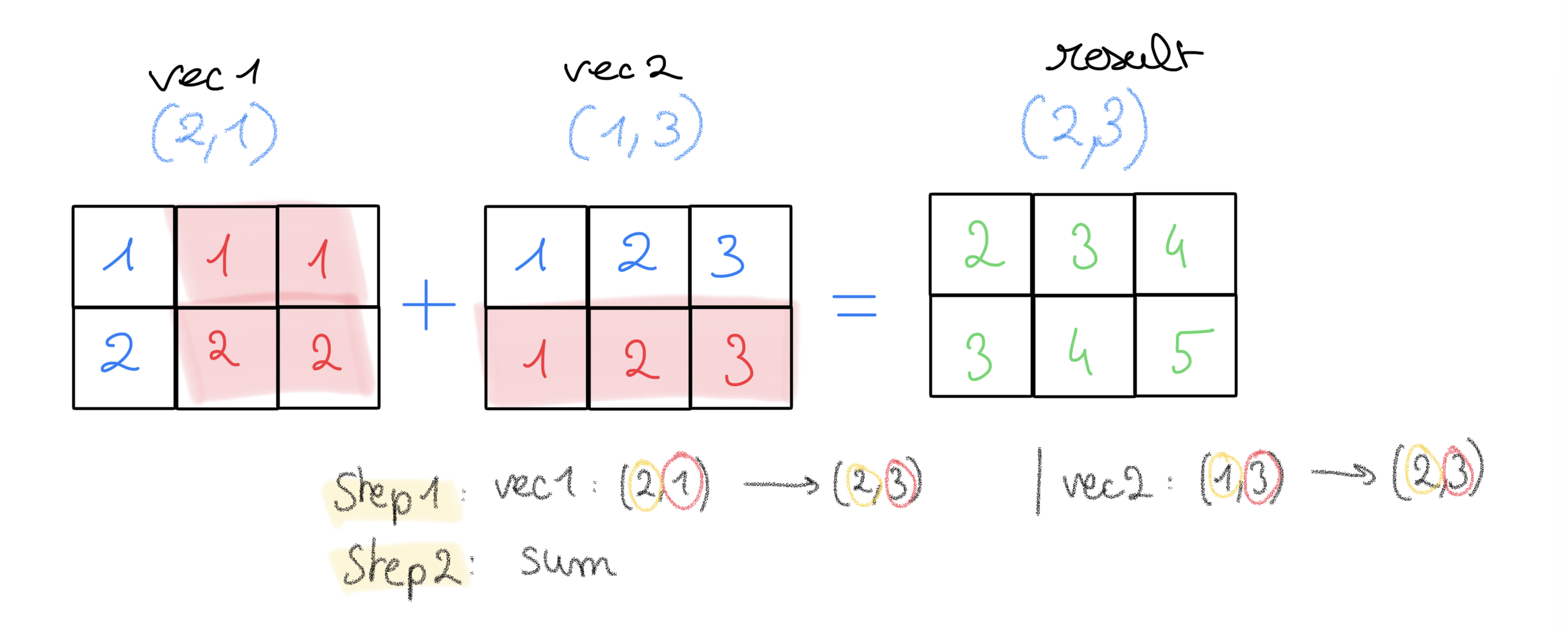
- 2 rows in
vector1,vector2does not have “rows dimension”, prepended a 1 to create a new dimension - then
vector2is stretched on its new dim so to have 2 elements, asvector1 - while
vector1has last dimensions (columns) strecthed to have 3 elements, asvector2
vector1 + vector2
array([[2, 3, 4],
       [3, 4, 5]])
This is the same as:
vector2
array([1, 2, 3])
np.tile(vector2, reps=(2, 1))
array([[1, 2, 3],
       [1, 2, 3]])
np.tile(vector1, reps=(1, 3))
array([[1, 1, 1],
       [2, 2, 2]])
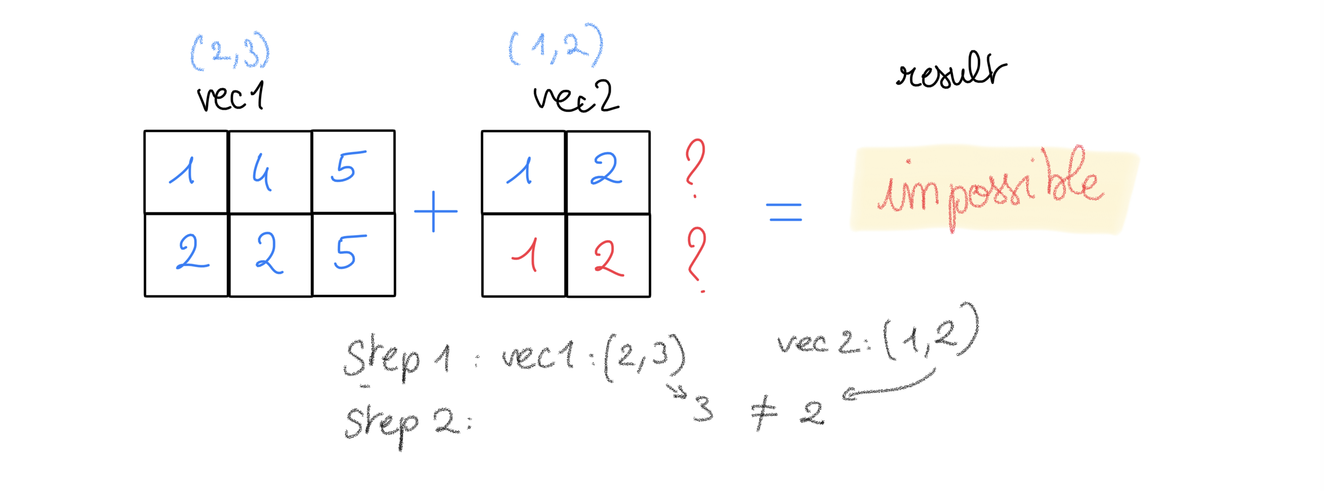
Example3:
vector1 = np.array([[1, 4, 5], [2, 2, 5]]) # 2 rows, 3 column
vector2 = np.array([1, 2]) # 1D vector
vector1.shape, vector2.shape
((2, 3), (2,))
try:
    vector1 + vector2
except Exception as e:
    print("After prepending with 1 the vector2, impossible to match 2 to 3:\n{}".format(e))
After prepending with 1 the vector2, impossible to match 2 to 3:
operands could not be broadcast together with shapes (2,3) (2,)
Another example:
Finding the parameters in a simple linear regression case
The data
%matplotlib inline
x = np.linspace(0, 100, 100)
y = 8*x + np.random.normal(x, 100) # y = 8*x + epsilon with epsilon ~ N(0,1)
plt.scatter(x, y)
plt.show()
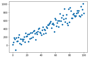
How to find the coefficient \(\beta\)s (here the intercept \(\beta\)0 and the slope \(\beta\)1) in order to have the best fitting (simple) linear model ?
The plotting function
def plotting(beta0, beta1):
    plt.scatter(x_scaled_and_centered, y)
    plt.plot(x_scaled_and_centered, beta0 + beta1 * x_scaled_and_centered, color='r')
Using OLS
from sklearn.linear_model import LinearRegression
# adding one dimension to the x (to have a feature matrix notation,
# although x is only 1 feature,
# which then can be apparented as a column vector
lm = LinearRegression().fit(x[:, np.newaxis], y)
lm.intercept_, lm.coef_
(37.18580177143173, array([8.22801749]))
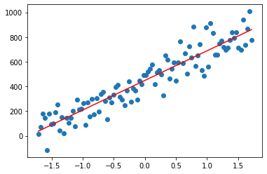
With standardization before:
from sklearn.preprocessing import StandardScaler
x_scaled_and_centered = StandardScaler().fit_transform(x[:, np.newaxis])
lm = LinearRegression(fit_intercept=True).fit(x_scaled_and_centerd, y)
lm.intercept_, lm.coef_
(448.5866764712714, array([239.90962559]))
plotting(lm.intercept_, lm.coef_)
Using a self-made (definitely non-optimised) algorithm
def algo_simple_linreg(x, y):
    """A self-made, definitely non-optimised algorithm to find the best alpha and beta values:"""
    from sklearn.metrics import mean_squared_error
    MSE = {}
    for beta0 in np.linspace(-5000, 5000, 100):
        for beta1 in np.linspace(-5000, 5000, 100):
            model = lambda x: beta0 + beta1*x
            mse = mean_squared_error( model(x), y)
            MSE[(beta0, beta1)] = mse
    return MSE
MSE = algo_simple_linreg(x_scaled_and_centered, y)
params = pd.Series(MSE).unstack()
import seaborn as sns
ax = plt.subplot(111)
sns.heatmap(params, cmap="coolwarm", ax=ax)
<AxesSubplot:>
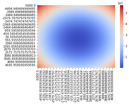
params.stack().idxmin()
(454.54545454545496, 252.52525252525265)
plotting(*params.stack().idxmin())

Using One neuron 🤓
Definition
2 nice definitions i like, just stolen from there
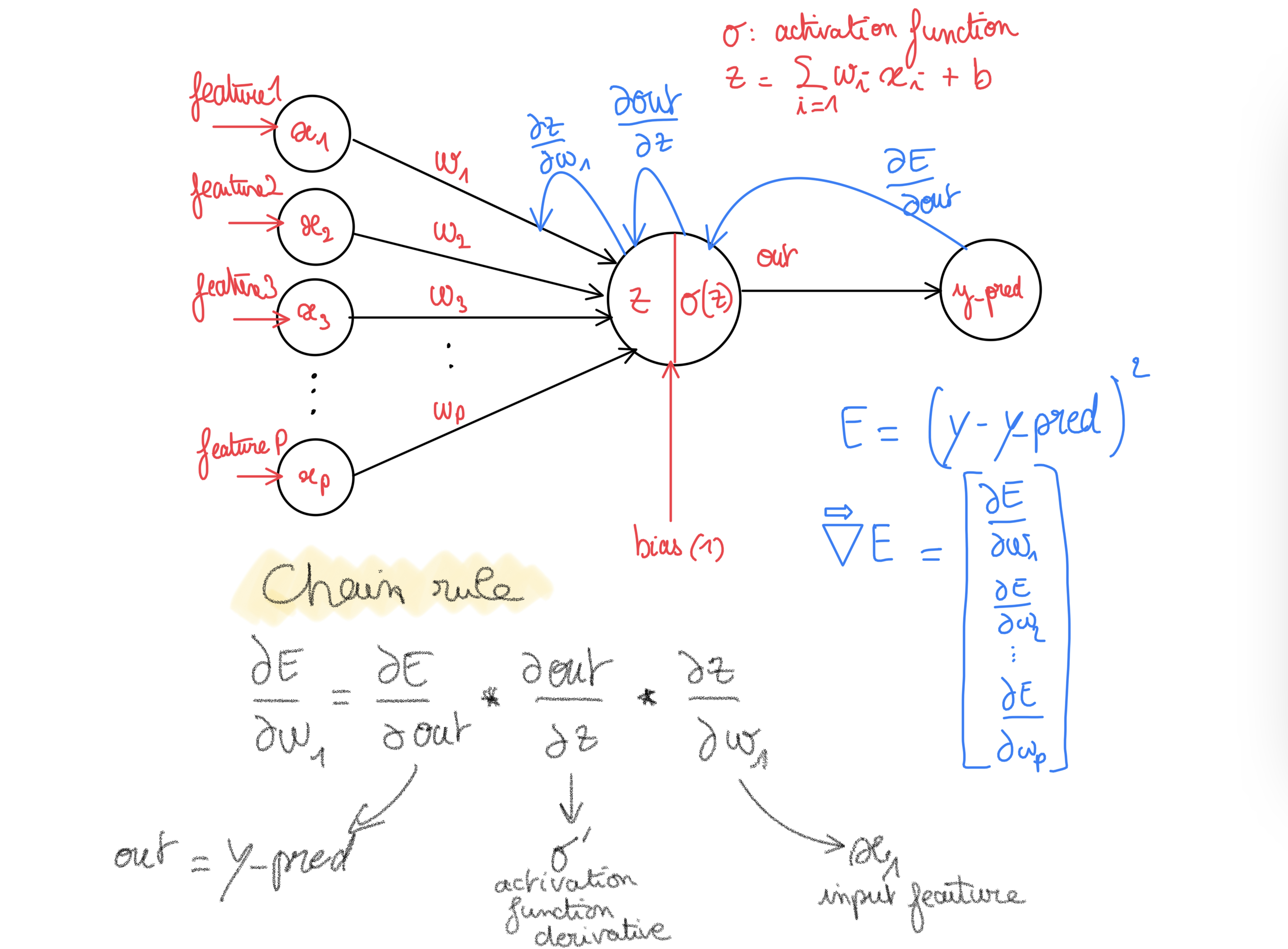
A processing “unit” applying a simple operation to its inputs, and which can be “connected” to others to build a network able to realize any input-output function
“Usual” definition: a “unit” computing a weighted sum of its inputs, that can add a constant term, and apply some non-linearity (sigmoïd, ReLU, …)
Behavior formulas
From the last definition of what a neuron is we get:
From the last definition of what a neuron is we get:
- Weighted sum of its inputs and can add a constant term. \(f(x_i) = \color{red}{\sum_{i=1}^{p}{w_i x_i}} + \color{blue}{cst}\)
- Apply some non-linearity function g:
Example: sigmoid function (g is Sigmoid) \(g(z) = Sigmoid(z) = \color{green}{\frac{1}{1+e^{-z}}}\)
Then the output of the neuron is: \(y_i = ( g \circ f ) (x) = g(f(x)) = \color{green}{\frac{1}{1+e^{-\color{red}{\sum_{i=1}^{p}{w_i x_i}} + \color{blue}{cst}}}}\)
Seems that 1. look very similar to a simple linear regression formula !
- The weights \(w_i\) can be seen as the coefficients of a linear regression.
- The \(x_i\) as the features of one data point (one row vector then i.e. one line of a matrix or one observation in a dataframe !). There is \(p\) features for one input vector here using the former notation.
- The output \(y_i\) is a scalar, that is, the output for one input vector of features \(i\)
We can rewrite this formula in vector notation, so we could scale this to multiple input vectors.
\[Y = (g \circ f) (X) = g( X W + B )\]or maybe using the indices so it is a little bit clearer
\[Y_{k,1} = (g \circ f) (X_{k,p}) = g( X_{k,p} W_{p,1} + B_{k,1} )\]Where \(X\) is a row vector of p features (or a matrix of n row vectors of p features).
This notation is useful as it could be used for one single input, or many.
- if one input row vector is passed, then, it is a simple dot product between this vector and a column weights vector occur, forming one scalar output \(Y_{1,1}\).
-
if multiple inputs are being passed (size \(k x p\)), then W is a matrix of size \(p x 1\) (for \(\hat{Y}\) being univariate or \(p x j\) if you want \(\hat{Y}\) to be a multivariate output of k rows/observations of j features each (one for each input)), forming finally a vector of outputs \(Y_{k,1}\).
- For a simple (1 feature) univariate (1 output) linear regression (no need of non-linear activation function) handled by a single neuron, the matrix of weights will be: \(W_{1,1}\). That is 1 single weight w1 so the formula is: \(\hat{y_i} = \hat{f}(x_{i,feature_1}) = w_1\*x_{i,feature_1})\)
- For a multiple (many features) univariate (1 output) linear regression (no need of non-linear activation function) handled by a single neuron, the matrix of weights will be \(W_{p,1}\). That is p weight (adapting to the p different features) and 1 single output (of activated(weighted sum + bias)).
Hence you can see the weight matrix does not depend of the number of data points, but on the number of features the data embed. You also have 1 added term/bias for each neuron, so the number of bias does not depend on the number of features but the number of neurons, and will be broadcasted to the number of data points (if you see the bias as an intercept, on each prediction you add the intercept of course).
In Python code,
the data:
# to set x as a matrix of row vectors of 1 feature each kx1
# for simple linear reg
x = x[:, np.newaxis]
the weight matrix:
W = np.random.random(size=(x.shape[1], 1))
# randomly generated weights
# depends on the number of features/cols in X
# 1xk for simple linear regression
# pxk for multiple one
# 1 col <=> 1 neuron <=> 1 output value (here we directly want y_pred)
and the bias term:
B = np.random.random(size=(x.shape[0], 1))
# one bias term for each neuron
# does not depend on the number of features in the data
# 1 neuron here -> as one single output variable y_pred,
# 1 bias then.
# it will be broadcoasted to the number of rows/data points
# hence applied on each input k (of 1 feature each)
Loss and Risk function
Remembered the cost function ?
Let’s take a quadratic loss as it is nicely differentiable,
Let’s write: \(z = (g \circ f)\)
then:
\[L(y_i, \hat{y_i}) = L(y_i, \hat{f}(x_i)) = (y_i - \hat{f}(x_i))^2\]Then in matrix notation:
\[L(Y_{k,1}, \hat{Y_{k,1}}) = L(Y_{k,1}, \hat{f}(X_{k,p}) = (Y_{k,1} - \hat{f}(X_{k,p}))^2\]Hence the result is a vector of loss for each output.
The cost function is the expected loss value, if we use the quadratic loss it then becomes the Mean Squared Error.
\[MSE = \frac{1}{n}\sum_{i=1}^{n}{ ( y_i - \hat{f}(x_i) )^2}\]and in matrix notation:
\[MSE = E[L(Y_{k,1}, \hat{Y}_{k,1})]= E[ (Y_{k,1} - \hat{f}(X_{k,p}))^2 ) ]\]Backpropagation
At first the weights (coefficients for a linear regression here) are chosen randomly.
Of course, if we knew them before, why would we use an algorithm ? :P
We are going to use Gradient descent: a first-order iterative optimization algorithm for finding a local minimum of a differentiable function. We want to minimize the produced errors, we will perform the gradient descent of the loss function. It implies computing the derivative of the loss function w.r.t. the weights. The quadratic loss function is then a good choice here as it is differentiable.
Computing the gradient of the loss function with respect to the weights enable us to later find (using the opposite) the direction in the weight/parameter space that minimizes the loss.
This derivative can be done in 2 different ways:
- each iteration can use one input vector. Each of the weights will be updated computing the derivative on the loss function w.r.t. the weights for that single input vector that had been passed forward to compute the output and so the errors, this is named: stochastic gradient descent.
- or each iteration can use a batch of multiple vectors (extreme case is using a bach that equals the training set, the whole data available, that is, k row vectors) to compute the expected loss value for that batch of inputs, this is named: batch gradient descent. This means that each weight will be updating by the one quantity meaned over the grouped information/directions from the predictions errors drawn from passing k input vectors.
Once computed, the gradient points uphill (maximize the loss), so we need to update the weights taking the opposite direction. Also we will carefully take each update a little step in this same direction by using the (negation of the) derivative by a coefficient also called learning rate: since it influences to what extent newly acquired information overrides old information (wikipedia always gives the best quote).
Following subsection gives the mathematical formulas of each of them.
Stochastic Gradient Descent (SGD)
For a (scalar) weight \(j\) associated to a feature number \(j\) (in simple linear regression, there would be only one anyway), the updating formula can be written as:
\[w_j = w_j - \alpha \frac{\partial L}{\partial w_j}\]Here L is the loss (hence computed on one input data point).
or in matrix notation for all the weights \(1...j...p\) for a single neuron (in a multiple linear regression framework):
\[W_{p,1} = W_{p,1} - \alpha \frac{\partial L}{\partial W_{p,1}}\]Here:
- at each iteration, to update of the weights we use one single data point as input.
- at each iteration, to update of the weights is driven by the prediction error made on that single input data point.
- at each iteration, the corresponding computation of the derivative of the loss of the prediction error for that data point serves as a basis to update all the weights in the weight (column) matrix W_{p,1}.
Batch or mini-batch Gradient Descent (BGD)
For a (scalar) weight \(j\) associated to a feature number \(j\):
\[w_j = w_j - \alpha \frac{\partial E}{\partial w_j}\]or in matrix notation for all the weights \(1... j... p\) for a single neuron (in our linear regression framework):
\[W_{p,1} = W_{p,1} - \alpha \frac{\partial E}{\partial W_{p,1}}\]Where E, for a batch, is the expected loss we want to differentiate (hence the MSE here since we took a quadratic loss):
\[W_{p,1} = W_{p,1} - \alpha \frac{\partial MSE}{\partial W_{p,1}}\] \[W_{p,1} = W_{p,1} - \alpha \frac{\partial \E[L(Y_{n,1}, \hat{Y_{n,1}})]}{\partial W_{p,1}}\]with \(n\) a grouped collection of n data points, also named a batch.
- \(n\) could be \(<= k\) the number of data points for the entire (training) dataset
- if \(n\) equals to \(k\), then the entire meaned predictions errors on the entire dataset as input has been used to drive the update process of each of the weights in the weight column matrix \(W_{p,1}\)
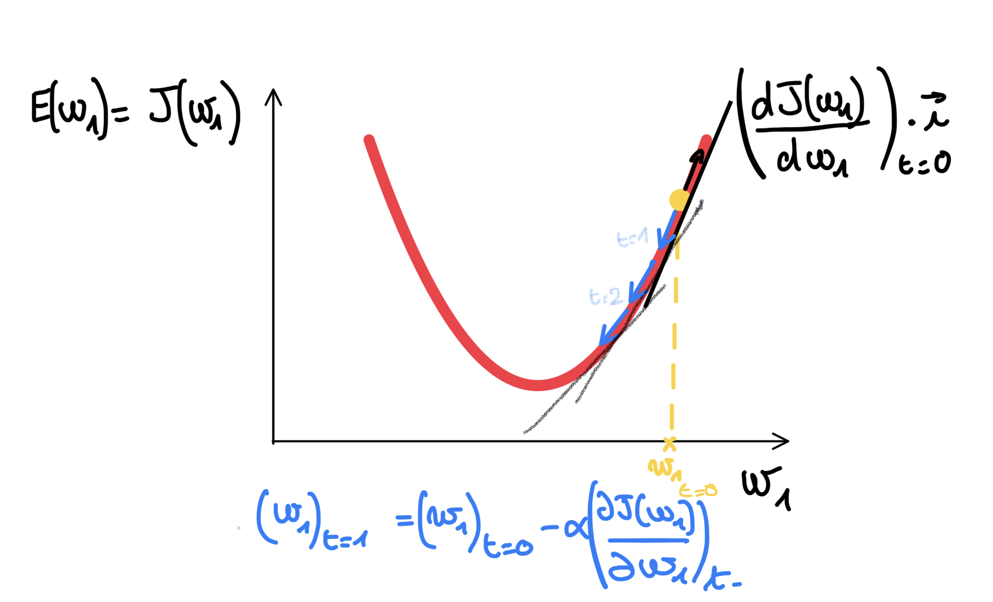
How to compute such gradient w.r.t. to the weights ? We use the chain rule !
from wikipedia: Intuitively, the chain rule states that knowing the instantaneous rate of change of z relative to y and that of y relative to x allows one to calculate the instantaneous rate of change of z relative to x.
As put by George F. Simmons: “if a car travels twice as fast as a bicycle and the bicycle is four times as fast as a walking man, then the car travels 2 × 4 = 8 times as fast as the man.”m
We are going to see how vary the prediction errors by making a change in the weight space (w.r.t. to each weight = gradient).
Here we face a composite function, as computing such derivative w.r.t one weight implies (using the chain rule):
- to first derive w.r.t the output of the activation function,
- then see how the output of the activation function changes w.r.t. the variable before the activation function (weighted inputs sum)
- then w.r.t. to the weight itself.
Recap
Here is just the same picture as before, so to always cross check everything is done right while creating the Neuron class for creating in the next section.

Time to implement it
which activation are we going to use ?
import numpy as np
import matplotlib.pyplot as plt
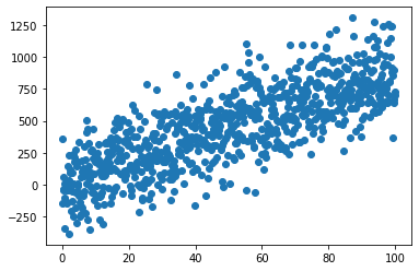
x = np.linspace(0, 100, 800)
y = 8*x + np.random.normal(x, 200) # y = 8*x + epsilon with epsilon ~ N(0,1)
plt.scatter(x, y)
plt.show()
x = x[:, np.newaxis] # to set x as a matrix of row vectors of 1 feature b
def split_n_batch_indexes(X, nb_chunks=5):
    import numpy as np
    indexes = np.arange(len(X))
    shuffled_indexes = np.random.shuffle(indexes)
    return np.array_split(indexes, nb_chunks)
class Neuron:
    """ Implementation of a single Neuron accepting multiple inputs """
    def __init__(self, X, y, nb_epochs=100, nb_batches=5,
                 learning_rate=0.01, activation="linear"):
        self.X, self.y = X, y
        # random weights
        self.W = np.random.random(size=(X.shape[1], 1))
        # random bias (only one as only one output)
        self.B = np.random.random(size=(1, 1))
        # number of epochs
        self.nb_epochs = nb_epochs
        # number of batches
        self.nb_batches = nb_batches
        # learning rate
        self.learning_rate = learning_rate
        # activation
        if activation=="linear":
            self.activation = lambda x: x
            self.derivative = lambda x: 1
        # records
        self.records = {}

    def forward_pass(self, is_batch):
        """ a single forward pass to compute a prediction """
        self.y_pred_batch = self.activation( self.X[is_batch] @ self.W + self.B)
        self.y_pred = self.activation( self.X @ self.W + self.B)

    def compute_mse_on_whole_dataset(self):
        """ return the mean squared errors on whole training set"""
        self.mse = np.mean((self.y - self.y_pred)**2)

    def backpropagation(self, is_batch):
        """ compute the gradient of the errors with respect to
        the weights using the chain rule """
        # gradient of the errors w.r.t the output/prediction
        dE_dout = 2*(self.y_pred_batch - self.y[is_batch, np.newaxis])
        # gradient of the prediction w.r.t before the activ. func
        dout_dz = self.derivative(self.X[is_batch]) #1 for linear
        # gradient of z w.r.t the weight
        dz_dw = self.X[is_batch]
        # final gradient w.r.t the weights:
        self.dE_dw = dE_dout * dout_dz * dz_dw
        # for the biases (only last part change)
        self.dE_db = dE_dout * dout_dz * 1

    def update_weights_and_biases(self):
        dE_dw = self.dE_dw.mean(axis=0)[:, np.newaxis]
        dE_db = self.dE_db.mean(axis=0)[:, np.newaxis]

        self.W = self.W - self.learning_rate * dE_dw
        self.B = self.B - self.learning_rate * dE_db


    def predict(self, X_test):
        """ same as forward pass, just provide our own X"""
        return self.activation( X_test @ self.W + self.B)

    def run(self):
        """ learn iteratively:
            - an iteration is a single forward and backward pass
            - an epoch is consumed when all the inputs from the
              dataset have been used for updating the weight and
              biases """
        # epochs
        for i in range(1, self.nb_epochs):
            # batches:
            for batch_i, indices in enumerate(
                    split_n_batch_indexes(self.X, self.nb_batches)):
                self.forward_pass(indices)
                self.compute_mse_on_whole_dataset()
                self.backpropagation(indices)
                self.update_weights_and_biases()
                self.records[(i, batch_i)] = [self.W, self.B, self.mse]
        return self.records
from sklearn.preprocessing import StandardScaler
from sklearn.model_selection import train_test_split
X_train, X_test, y_train, y_test = train_test_split(x, y)
scaler = StandardScaler().fit(X_train)
X_train = scaler.transform(X_train)
X_test = scaler.transform(X_test)
neuron = Neuron(X_train, y_train)
neuron
<__main__.Neuron at 0x12d97f9a0>
records = neuron.run()
import pandas as pd
index = pd.MultiIndex.from_tuples(records.keys())
records = pd.DataFrame(records.values(),
            index=index,
            columns=['weights', 'bias', 'mse_train'])
records
| weights | bias | mse_train | ||
|---|---|---|---|---|
| 1 | 0 | [[4.443509449033136]] | [[9.644383787235665]] | 316078.087993 |
| 1 | [[10.21384857348198]] | [[18.956325297600568]] | 307829.453673 | |
| 2 | [[13.829465261075233]] | [[27.481262123908465]] | 299653.437801 | |
| 3 | [[18.483634718716814]] | [[35.58832870180558]] | 292329.983030 | |
| 4 | [[24.778160591422168]] | [[44.41565823450879]] | 285568.062128 | |
| ... | ... | ... | ... | ... |
| 99 | 0 | [[257.33337321955196]] | [[457.91336158008875]] | 173202.046267 |
| 1 | [[256.7620263257349]] | [[457.9678800130618]] | 173143.006457 | |
| 2 | [[256.873731154326]] | [[457.78357255910817]] | 172849.289663 | |
| 3 | [[257.1059056991105]] | [[457.45374334250926]] | 172906.655320 | |
| 4 | [[257.4797445493716]] | [[457.8868223084108]] | 173026.140104 |
495 rows × 3 columns
df_weights = records.weights.apply(np.ravel).apply(pd.Series)
df_bias = records.bias.apply(np.ravel).apply(pd.Series)
df_bias.rename(columns = lambda x: "bias_{}".format(x), inplace=True)
df_weights.rename(columns = lambda x: "weights_{}".format(x), inplace=True)
df = pd.concat([df_weights, df_bias], axis=1)
df
| weights_0 | bias_0 | ||
|---|---|---|---|
| 1 | 0 | 4.443509 | 9.644384 |
| 1 | 10.213849 | 18.956325 | |
| 2 | 13.829465 | 27.481262 | |
| 3 | 18.483635 | 35.588329 | |
| 4 | 24.778161 | 44.415658 | |
| ... | ... | ... | ... |
| 99 | 0 | 257.333373 | 457.913362 |
| 1 | 256.762026 | 457.967880 | |
| 2 | 256.873731 | 457.783573 | |
| 3 | 257.105906 | 457.453743 | |
| 4 | 257.479745 | 457.886822 |
495 rows × 2 columns
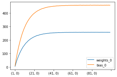
df.plot(kind="line")
/Users/lucbertin/.pyenv/versions/3.8.4/lib/python3.8/site-packages/pandas/plotting/_matplotlib/core.py:1235: UserWarning: FixedFormatter should only be used together with FixedLocator
  ax.set_xticklabels(xticklabels)


<AxesSubplot:>
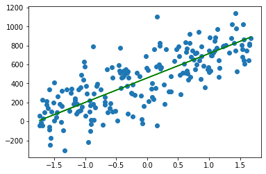
plt.scatter(X_test, y_test)
plt.plot(X_test, neuron.predict(X_test), color='green')
[<matplotlib.lines.Line2D at 0x12df02610>]
%matplotlib notebook

import matplotlib.animation as animation

fig, ax = plt.subplots()
# Initial plot
x_ = np.linspace(-2, 2, 100).reshape((100,1))
# y_ = weight*x_ + bias
y_ = float(df.iloc[0, 0])*x_ + float(df.iloc[0, 1])

line, = ax.plot(x_, y_, label="Fit from the neuron")

plt.rcParams["figure.figsize"] = (4,2)
plt.ylabel("y")
plt.xlabel("X")
plt.scatter(X_train, y_train, color='red', label="Training data")
plt.scatter(X_test, y_test, color='green', label="Test data")
plt.xlim(-2, 2)
plt.legend()
plt.title("Linear regression training fit using a single neuron | perceptron")

def animate(i):
    line.set_label("Fit from the perceptron : epoch {}".format(i))
    plt.legend()
    x_ = np.linspace(-2, 2, 100).reshape((100,1))
    line.set_xdata(x_)  # update the data
    line.set_ydata( float(df.iloc[i, 0])*x_
                   + float(df.iloc[i, 1]))# update the data
    return line,

ani = animation.FuncAnimation(fig, animate, frames=np.arange(1, len(df)), interval=100)
plt.show()
<IPython.core.display.Javascript object>
Let’s try with multiple features ;-)
OLS
from sklearn.datasets import load_boston
from sklearn.preprocessing import StandardScaler
from sklearn.linear_model import LinearRegression
from sklearn.model_selection import train_test_split
X, y = load_boston(return_X_y=True)
X_train, X_test, y_train, y_test = train_test_split(X, y, test_size=0.2)
scaler  = StandardScaler()
X_train = scaler.fit_transform(X_train)
X_test  = scaler.transform(X_test)
lm = LinearRegression().fit(X_train, y_train)
print( "linear regression coefficients {}".format(lm.coef_) )
linear regression coefficients [-0.72097319  1.32905744  0.14098068  0.31901842 -1.9611038   2.39122944
  0.02842854 -3.10284546  2.2339583  -1.52408631 -1.94909087  1.18566169
 -3.79786679]
With our Neuron
neuron_on_boston = Neuron(X_train, y_train,
                          learning_rate=0.1,
                          nb_batches=1)
records_on_boston = neuron_on_boston.run()
import pandas as pd
index = pd.MultiIndex.from_tuples(records_on_boston.keys())
df_boston = pd.DataFrame(records_on_boston.values(),
            index=index, columns=['weights', 'bias', 'mse_train'])
df_weights = df_boston.weights.apply(np.ravel).apply(pd.Series)
df_bias = df_boston.bias.apply(np.ravel).apply(pd.Series)
df_bias.rename(columns = lambda x: "bias_{}".format(x), inplace=True)
df_weights.rename(columns = lambda x: "weights_{}".format(x), inplace=True)
df = pd.concat([df_weights, df_bias], axis=1)
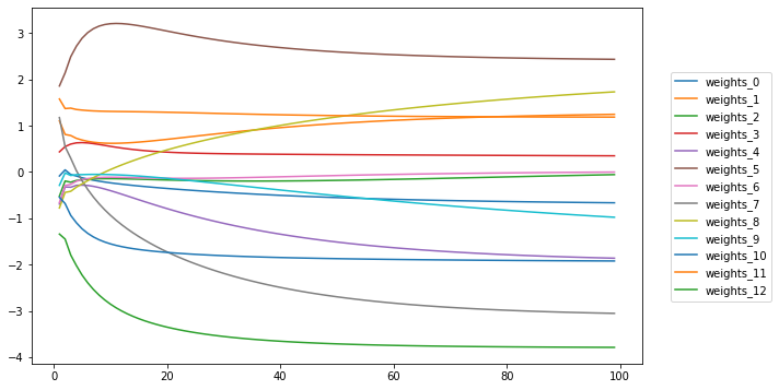
%matplotlib inline
fig = plt.Figure(figsize=(10,6))
ax = fig.gca()
save = df.drop("bias_0", axis=1).stack().unstack(level=0).loc[0].T
save.plot(ax=ax)
ax.legend().remove()
fig.legend(loc='center', bbox_to_anchor=(1,0.5))
fig
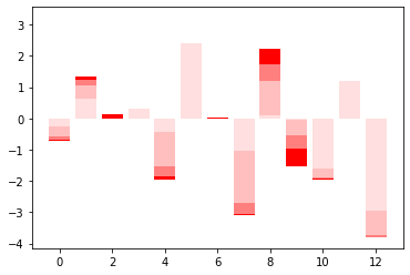
at_10  = save.iloc[10]
at_50 = save.iloc[50]
at_98 = save.iloc[98]
plt.bar(x=np.arange(len(lm.coef_)), height=lm.coef_, color='red')
plt.bar(x=np.arange(len(lm.coef_)), height=at_10, color='white', alpha = 0.5)
plt.bar(x=np.arange(len(lm.coef_)), height=at_50, color='white', alpha = 0.5)
plt.bar(x=np.arange(len(lm.coef_)), height=at_98, color='white', alpha = 0.5)
<BarContainer object of 13 artists>
Add-on: using Keras ?
from keras.models import Sequential
from keras.layers import Dense
from keras import optimizers
import pandas as pd
model = Sequential()
model.add(Dense(1, input_shape=(X.shape[1],), activation='linear'))
sgd = optimizers.SGD(lr=0.02)
model.compile(loss='mean_squared_error', optimizer=sgd)
A callback to store weights
from keras.callbacks import LambdaCallback

weights = {}
def save_weights(epoch, logs):
    weights[epoch] = model.layers[0].get_weights()

keep_weights = LambdaCallback(on_epoch_end=save_weights)
history = model.fit(x=X_train, y=y_train,
                    batch_size=X_train.shape[0], epochs=99,
                    validation_data=(X_test, y_test),
                    verbose=0, callbacks=[keep_weights])
print(history.params)
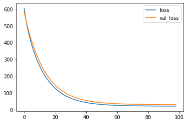
losses_ = pd.DataFrame(history.history)
losses_.plot(kind="line")
{'verbose': 0, 'epochs': 99, 'steps': 1}


<AxesSubplot:>
df_weights = pd.DataFrame(weights).T
coefs_linear_reg = dict(zip(
    ["weight_{}".format(_) for _ in range(len(lm.coef_))],
    lm.coef_
))
coefs_linear_reg
{'weight_0': -0.720973185445283,
 'weight_1': 1.3290574386023888,
 'weight_2': 0.14098068438146516,
 'weight_3': 0.3190184199461178,
 'weight_4': -1.9611038002705747,
 'weight_5': 2.3912294381194052,
 'weight_6': 0.028428542130489065,
 'weight_7': -3.1028454604117153,
 'weight_8': 2.2339582985686506,
 'weight_9': -1.5240863072636608,
 'weight_10': -1.949090868280713,
 'weight_11': 1.1856616926433907,
 'weight_12': -3.797866790151385}
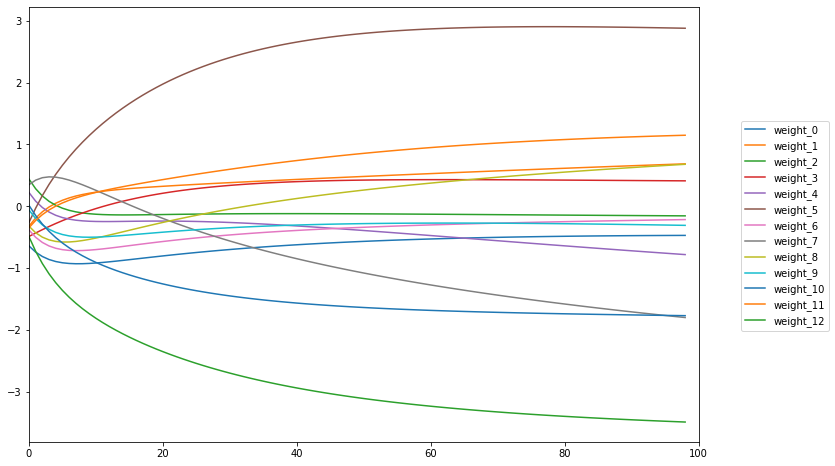
fig, ax = plt.subplots(figsize=(12,8))
( df_weights[0]
     .apply(np.ravel)
     .apply(pd.Series)
     .rename(columns = lambda x: "weight_{}".format(x))
     .plot(kind='line', ax=ax) )
ax.set_xlim(0,100)
ax.legend().remove()
fig.legend(loc='center', bbox_to_anchor=(1, 0.5))
<matplotlib.legend.Legend at 0x14e6d2be0>
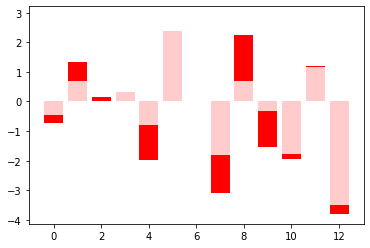
at_98  = df_weights.iloc[98,0].reshape(-1)
plt.bar(x=np.arange(len(lm.coef_)), height=lm.coef_, color='red')
plt.bar(x=np.arange(len(lm.coef_)), height=at_98, color='white', alpha = 0.8)
#history.model.get_weights()
<BarContainer object of 13 artists>
Bonus
Un lien sympathique pour s’amuser avec différentes architectures de réseau de neurones.

 Supervised Machine Learning