Binary classification - Titanic Dataset - Quick example

This is a classification scenario where you try to predict a categorical binary target y if the person survived (1) or not (0) from the Titanic.
This example is really short and here just to cover an example of classification as we mainly focused on regression so far.
Most of the supervised learning workflow does not change. You will most likely use classifier estimators from scikit, can also pick a different loss function, and a global metric that is most suited for your use-case.

url = 'https://gist.githubusercontent.com/michhar/2dfd2de0d4f8727f873422c5d959fff5/raw/fa71405126017e6a37bea592440b4bee94bf7b9e/titanic.csv'

First imports

Some may be added along with this practice session

import matplotlib.pyplot as plt
import seaborn as sns
import pandas as pd
import numpy as np

Download the dataset

using shell command wget

!wget -O montitanic.csv $url

pandas.read_csv can also read directly from a URL

pd.set_option("max_rows", 100) # just for showing more lines by default

df = pd.read_csv(url)
df.head(3)

	PassengerId	Survived	Pclass	Name	Sex	Age	SibSp	Parch	Ticket	Fare	Cabin	Embarked
0	1	0	3	Braund, Mr. Owen Harris	male	22.0	1	0	A/5 21171	7.2500	NaN	S
1	2	1	1	Cumings, Mrs. John Bradley (Florence Briggs Th...	female	38.0	1	0	PC 17599	71.2833	C85	C
2	3	1	3	Heikkinen, Miss. Laina	female	26.0	0	0	STON/O2. 3101282	7.9250	NaN	S

Health checks

Checking the documentation of the dataset

The target

• y = survived indicator (0 No, 1 yes)

The features

• Pclass = passenger class: 1st class, 2nd class, 3rd class
• name = name of the person
• sex
• age
• sibsip = number of siblings/spouses who traveled with the person
• parch = number of parents (children?) who traveled with the person
• ticket = ticket number / identifier
• fare = ticket price in pounds
• cabin = cabin type
• embarked = ferry port / jetty

Checks on the dataset

nb of rows / columns

df.shape

(891, 12)

Checking the columns

df.columns

Index(['PassengerId', 'Survived', 'Pclass', 'Name', 'Sex', 'Age', 'SibSp',
       'Parch', 'Ticket', 'Fare', 'Cabin', 'Embarked'],
      dtype='object')

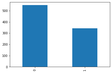
Checking the proportion of each values the binary target can take

df.Survived.value_counts() # the target = y, imbalanced/balanced dataset ?

0    549
1    342
Name: Survived, dtype: int64

df.Survived.value_counts().plot(kind="bar")

<AxesSubplot:>

infered types of each column

df.dtypes

PassengerId      int64
Survived         int64
Pclass           int64
Name            object
Sex             object
Age            float64
SibSp            int64
Parch            int64
Ticket          object
Fare           float64
Cabin           object
Embarked        object
dtype: object

Categorical vs Numerical Features

which features are categorical ? numerical ?

• categorical: Sex, Name, titleName, Embarked, Ticket
  • ordinal: Pclass
• numerical:
  • continuous=Age, Fare
  • discrete=SibSp, Parch

The outcome variable y is categorical

categorical_cols = ["Sex", "Embarked", "Pclass", "Cabin", "Ticket"] 
numerical_cols = ["Age", "Fare", "SibSp", "Parch"]

Let’s convert categorical columns as is

df[categorical_cols] = df[categorical_cols].astype("category")
df.dtypes

PassengerId       int64
Survived          int64
Pclass         category
Name             object
Sex            category
Age             float64
SibSp             int64
Parch             int64
Ticket         category
Fare            float64
Cabin          category
Embarked       category
dtype: object

len(categorical_cols ) + len(numerical_cols)

9

set(df.columns) - set(categorical_cols + numerical_cols)

{'Name', 'PassengerId', 'Survived'}

number of unique values for each column

df.nunique()

PassengerId    891
Survived         2
Pclass           3
Name           891
Sex              2
Age             88
SibSp            7
Parch            7
Ticket         681
Fare           248
Cabin          147
Embarked         3
dtype: int64

df.drop("Ticket", axis=1, inplace=True)
categorical_cols.remove("Ticket")

an easy-win: df.describe()

df[numerical_cols].describe()

	Age	Fare	SibSp	Parch
count	714.000000	891.000000	891.000000	891.000000
mean	29.699118	32.204208	0.523008	0.381594
std	14.526497	49.693429	1.102743	0.806057
min	0.420000	0.000000	0.000000	0.000000
25%	20.125000	7.910400	0.000000	0.000000
50%	28.000000	14.454200	0.000000	0.000000
75%	38.000000	31.000000	1.000000	0.000000
max	80.000000	512.329200	8.000000	6.000000

df[categorical_cols].describe()

	Sex	Embarked	Pclass	Cabin
count	891	889	891	204
unique	2	3	3	147
top	male	S	3	B96 B98
freq	577	644	491	4

Preprocessing (example)

Let’s try to extract the sexe gender of a person based on his name and cross-check with the sex column.

df['titleName'] = df.Name.str.extract("(?i)(mrs|mr|miss)")

print( df.loc[df.Sex == "male", "titleName"].isin(["miss", "mrs"]).any() )
print( df.loc[df.Sex == "female", "titleName"].isin(["mr"]).any() )

False
False

Good thing here, the sex type is matching the particle in the name (Mr = male, Miss and Mrs = female)

df.titleName.isna().mean() *100

7.182940516273851

Though, there is still 7% of missing values from the transformation of the name, let’s further check this.m

We see the particle is always followed by a dot, let’s try to extract it this way then.

df["titleName"] = df.Name.str.extract("([a-zA-Z]+)\.")
df.titleName.value_counts().plot(kind="bar")

<AxesSubplot:>

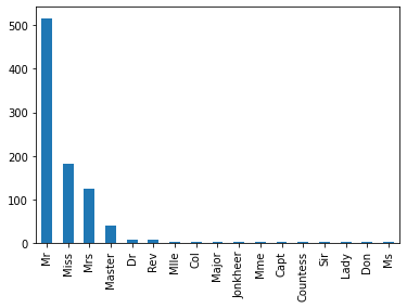
Mr, Miss and Mrs are the most represented titleName.
Let’s check with all the different values’ proportions.

labels = df.titleName.value_counts()
labels

Mr          517
Miss        182
Mrs         125
Master       40
Dr            7
Rev           6
Mlle          2
Col           2
Major         2
Jonkheer      1
Mme           1
Capt          1
Countess      1
Sir           1
Lady          1
Don           1
Ms            1
Name: titleName, dtype: int64

Some labels/titleName are really minorities. Let’s regroup them in “other”.

df.loc[df.titleName.isin(labels[labels<10].index), "titleName"] = "other"

Adding to the categorical columns:

categorical_cols.append('titleName')

Some other Exploratory Data Analysis

ticket prices distribution

df.Fare.min()

0.0

df.Fare.plot(kind="density", xlim=(df.Fare.min(), df.Fare.max()))

<AxesSubplot:ylabel='Density'>

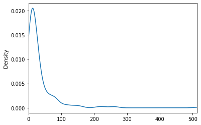
highly right-skewed, who paid so much ?

df.loc[ df.Fare == df.Fare.max()]

	PassengerId	Survived	Pclass	Name	Sex	Age	SibSp	Parch	Fare	Cabin	Embarked	titleName
258	259	1	1	Ward, Miss. Anna	female	35.0	0	0	512.3292	NaN	C	Miss
679	680	1	1	Cardeza, Mr. Thomas Drake Martinez	male	36.0	0	1	512.3292	B51 B53 B55	C	Mr
737	738	1	1	Lesurer, Mr. Gustave J	male	35.0	0	0	512.3292	B101	C	Mr

who does not pay anything for onboarding ?

df.loc[ df.Fare == df.Fare.min()]

	PassengerId	Survived	Pclass	Name	Sex	Age	SibSp	Parch	Fare	Cabin	Embarked	titleName
179	180	0	3	Leonard, Mr. Lionel	male	36.0	0	0	0.0	NaN	S	Mr
263	264	0	1	Harrison, Mr. William	male	40.0	0	0	0.0	B94	S	Mr
271	272	1	3	Tornquist, Mr. William Henry	male	25.0	0	0	0.0	NaN	S	Mr
277	278	0	2	Parkes, Mr. Francis "Frank"	male	NaN	0	0	0.0	NaN	S	Mr
302	303	0	3	Johnson, Mr. William Cahoone Jr	male	19.0	0	0	0.0	NaN	S	Mr
413	414	0	2	Cunningham, Mr. Alfred Fleming	male	NaN	0	0	0.0	NaN	S	Mr
466	467	0	2	Campbell, Mr. William	male	NaN	0	0	0.0	NaN	S	Mr
481	482	0	2	Frost, Mr. Anthony Wood "Archie"	male	NaN	0	0	0.0	NaN	S	Mr
597	598	0	3	Johnson, Mr. Alfred	male	49.0	0	0	0.0	NaN	S	Mr
633	634	0	1	Parr, Mr. William Henry Marsh	male	NaN	0	0	0.0	NaN	S	Mr
674	675	0	2	Watson, Mr. Ennis Hastings	male	NaN	0	0	0.0	NaN	S	Mr
732	733	0	2	Knight, Mr. Robert J	male	NaN	0	0	0.0	NaN	S	Mr
806	807	0	1	Andrews, Mr. Thomas Jr	male	39.0	0	0	0.0	A36	S	Mr
815	816	0	1	Fry, Mr. Richard	male	NaN	0	0	0.0	B102	S	Mr
822	823	0	1	Reuchlin, Jonkheer. John George	male	38.0	0	0	0.0	NaN	S	other

Proportion of each value each categorical feature may take

categorical_cols.remove('Cabin') # we will explain why later on

n = len(categorical_cols)

fig, axes = plt.subplots(1, n, figsize=(15, 4), sharey=True)
for i, colname in enumerate(categorical_cols):
    sns.countplot(x=colname, data=df, ax=axes[i])

and with respect to the target

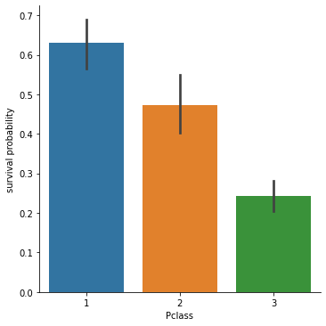
From the next plot we can see that the Survival probability is linked with the membership to a Pclass value.

sns.catplot(x="Pclass", y="Survived", kind="bar", data=df).set_ylabels("survival probability")

<seaborn.axisgrid.FacetGrid at 0x178b37220>

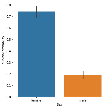
But also to the sex category of a person.

sns.catplot(x="Sex", y="Survived", kind="bar", data=df).set_ylabels("survival probability")

<seaborn.axisgrid.FacetGrid at 0x178b0e040>

We may want to further quantify this relationship using statistical tests.

Let’s keep our investigations going on.

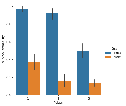
Trying to check the influence of both features on the survival problability (does a female in 3rd class had more chance to survive to the Titanic compared to a male on 1st class ?)

sns.catplot(x="Pclass", y="Survived", hue="Sex", kind="bar", data=df).set_ylabels("survival probability")

<seaborn.axisgrid.FacetGrid at 0x178bd0fd0>

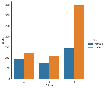
And let’s also check the number of people constituing each of those subgroups.

sns.catplot(x="Pclass",hue="Sex", kind="count", data=df)

<seaborn.axisgrid.FacetGrid at 0x178c499d0>

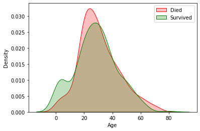
Did the age have a correlation with the chance of survival ?

plot = sns.kdeplot(df.loc[ df.Survived == 0, "Age"], color="Red", shade=True)
plot = sns.kdeplot(df.loc[ df.Survived == 1, "Age"], color="Green", shade=True)
plot.legend(["Died", "Survived"])

<matplotlib.legend.Legend at 0x178ccfa90>

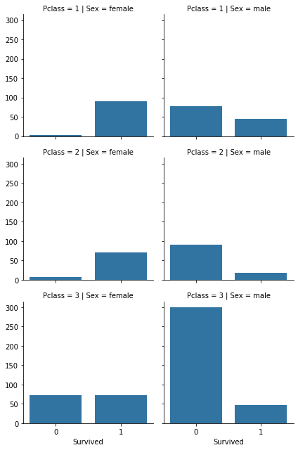
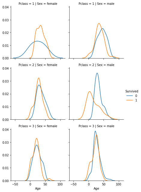
2 other plots (try to reproduce them):

• number of people for survivor and deceased person w.r.t. their Pclass and sex category
• distribution of ages for survivor and deceased person w.r.t their Pclass and sex

Missing values ?

df.isna().sum()

PassengerId      0
Survived         0
Pclass           0
Name             0
Sex              0
Age            177
SibSp            0
Parch            0
Fare             0
Cabin          687
Embarked         2
titleName        0
dtype: int64

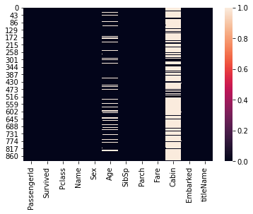
Graphically (can be nice to see if some missing values in a column have corresponding missing values in other columns).

sns.heatmap(df.isna())

<AxesSubplot:>

1. Handling missing values in Cabin column

df.Cabin.isna().sum()

687

df.Cabin.nunique()

147

a lot of unique different labels for Cabin + a lot of missing values for Cabin.

(687 + 147) / df.shape[0] * 100 # in %

93.60269360269359

df.drop("Cabin", axis=1, inplace=True)

2. Handling missing values in Embarked column

df.Embarked.isna().sum()

2

df.Embarked.value_counts()

S    644
C    168
Q     77
Name: Embarked, dtype: int64

df.Embarked.value_counts()[df.Embarked.mode()] / df.Embarked.value_counts().sum() *100

S    72.440945
Name: Embarked, dtype: float64

S level account for 72% of the values in the dataset.

Let’s replace the missing value by the mode (they are only 2 missing values in df.Embarked)

df.Embarked.fillna(df.Embarked.mode()[0], inplace=True)

df.Embarked.value_counts()

S    646
C    168
Q     77
Name: Embarked, dtype: int64

3. Handling missing values in Age column

sns.displot(df.Age, kde=True)

<seaborn.axisgrid.FacetGrid at 0x178cb5040>

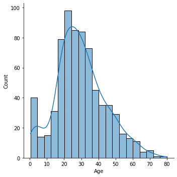
Replacing the age by the mean in the entire population is really a strong assumption, but i don’t want to put too much emphasis on this part.

df.Age.fillna(df.Age.mean(), inplace=True) 

Modelling

final processing before injecting roughly in the model

df.drop("PassengerId", axis=1, inplace=True)
df.drop("Name", axis=1, inplace=True)
df.drop('flag', axis=1, inplace=True)

separating the target from the feature matrix:

X, y = df.drop("Survived", axis=1), df.Survived

encoding the categorical features

Some ML algorithm can’t accept non-encoded features as such.

• the Pclass is an ordinal variable (1st class > 2nd class > 3rd class)

from sklearn.preprocessing import OrdinalEncoder
encoder = OrdinalEncoder()
X[["Pclass"]] = encoder.fit_transform(X[["Pclass"]])
encoder.categories_

[array([1, 2, 3])]

• the sex column is not.
  because there is no apparent ordering between male and female (e.g. can we say male > female or female > male ?)
  same for Embarked and titleName (although we could argue about the later)

from sklearn.preprocessing import OneHotEncoder
encoder = OneHotEncoder(drop="first", sparse=False)
X[encoder.get_feature_names(["is", "embarked_from", "hastitle"])] =\
    encoder.fit_transform(X[["Sex" , "Embarked", "titleName"]])
X.drop(["titleName", "Embarked", "Sex"], axis=1, inplace=True)

X.head()

	Pclass	Age	SibSp	Parch	Fare	is_male	embarked_from_Q	embarked_from_S	hastitle_Miss	hastitle_Mr	hastitle_Mrs	hastitle_other
0	2.0	22.0	1	0	7.2500	1.0	0.0	1.0	0.0	1.0	0.0	0.0
1	0.0	38.0	1	0	71.2833	0.0	0.0	0.0	0.0	0.0	1.0	0.0
2	2.0	26.0	0	0	7.9250	0.0	0.0	1.0	1.0	0.0	0.0	0.0
3	0.0	35.0	1	0	53.1000	0.0	0.0	1.0	0.0	0.0	1.0	0.0
4	2.0	35.0	0	0	8.0500	1.0	0.0	1.0	0.0	1.0	0.0	0.0

Applying some models

from sklearn.model_selection import train_test_split
X_train, X_test, y_train, y_test = train_test_split(X, y, test_size=0.2)

from sklearn.linear_model import LogisticRegression
logreg = LogisticRegression(max_iter=1000)
logreg.fit(X_train, y_train)

LogisticRegression(max_iter=1000)

Let’s have a look at one metric: the accuracy

from sklearn.metrics import accuracy_score
accuracy_score(y_true=y_test, y_pred=logreg.predict(X_test))

0.776536312849162

doesn’t seem that bad, but… think again about the dataset itself and the proportion of each values y take.

from sklearn.metrics import plot_confusion_matrix
plot_confusion_matrix(logreg, X=X_test, y_true=y_test) # accept an already fitted model

<sklearn.metrics._plot.confusion_matrix.ConfusionMatrixDisplay at 0x1793eb490>

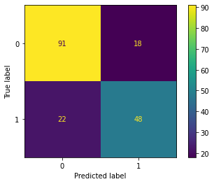
Accuracy is defined as the sum of the diagonal elements over the sum of all the elements of the confusion matrix.

In other words, which proportion of the observed y values match with the predictions made by the model, no matter what class (positive / negative) y belong too.

accuracy = (91+48)/(22+18+91+48)
accuracy

0.776536312849162

if we took a very extreme example where our model is “dummy” and only output y as died: then accuracy would be:

y_test.value_counts()[0]  / y_test.value_counts().sum() *100

60.893854748603346

61%

Now, imagine we had 99% of people dying in the test set, the accuracy of this dummy model would raise up to 99 !.

Hence you should try to check some other metrics depending on the use-case, and/or the business mater, and/or whether you are in case of imbalanced dataset.

It often boils down to a trade-off:

• do you want to detect any true case of survival (y_pred = y_obs = 1) ? at the expense of predicting people as survivor (y_pred = 1) when they were actually observed as dead (y_obs = 0). This is also named a false positive.
  • This case scenario would be a good use-case if we wanted to detect if someone could possibly have a rare disease. We would prefer the test to be overly detecting a disease even when the patient isn’t affected by any disease (y_obs=0 and y_pred=1): the patient could procede further tests to ensure it does not have the disease.
• or do you prefer to detect any true case of death (y_pred = y_obs = 0)? at the expense of classifying people as dead (y_pred = 0) when they were actually observed as survivor (y_obs = 1). This is also named a false negative.
  • This case scenario would be a good use-case for spams detection. We certainly would want to detect spams, but one person may find it very annoying the emails he sends to people are flagged as spam by the AI engine (y_pred=1) when it is clearly not (y_obs=0). So we even more want to prevent this from happening.

Of course in theory you could have a perfect model which does not create neither false positive, nor false negative, and output an accuracy of 100%. But this is not so often in practice.

Note that some metrics represent either of those scenarii, or combine (with some weighted proportion) a mix of both. I leave this to you as an exercice to find which is best suited to your problem..

Final words

• For the rest of this exercice you can try other models, once you have defined which metrics you want to assess your model performance.
• You can reuse the model validation techniques we used in other lessons (k-fold, gridsearch, learning curves, etc.)