Some regressions on some data

In this hands-on session, we will be using some well-known machine learning models for regression purposes. I said “regression” because we will be trying to predict a (random) variable Y designing a numerical quantity.

Imports

We first import the common packages for data processing and visualization:

# general import for data treatment and visualization
import numpy as np
import pandas as pd
import matplotlib.pyplot as plt
import seaborn as sns
import imageio
# models we will be using
from sklearn.linear_model import LinearRegression
from sklearn.tree import DecisionTreeRegressor, plot_tree
from sklearn.ensemble import RandomForestRegressor
from sklearn.neighbors import KNeighborsRegressor
# model validation techniques
from sklearn.model_selection import train_test_split
from sklearn.model_selection import cross_val_score, cross_val_predict
from sklearn.model_selection import GridSearchCV
from sklearn.model_selection import KFold
from matplotlib import gridspec
# mse: metric used
from sklearn.metrics import mean_squared_error, make_scorer

Problem 1: data modeled using a linear model

The data

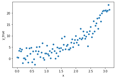
We will generate data from a supposedly unobservable function that we will try to approximate.

The function is expressed as: \(f(x) = e^x\)

Let’s add some random noise following a gaussian distribution with conditional mean of 0 (strong endogeneity i.e. there is no leakage of information posed by independent variables into the error term).

data = pd.DataFrame(dict(
    x = np.linspace(0, np.pi, 100),
    y_true = np.random.normal(np.exp(x), scale=2.0)))

Separating in X (a matrix of one single column = feature = independent variable) and y…

df, y = data.drop("y_true", axis=1), data.y_true

fig = plt.Figure()
sns.scatterplot(x="x", y=y, data=df, ax=fig.gca())
fig

Linear regression model

Statistical population model

Let’s first assume a linear relationship between y and the matrice X of (1) feature(s), using a linear regression model.

\[y = \beta_0 + \beta_1x_1 + \beta_2 x_2 + ... \beta_n x_n + \epsilon_i\]

with \(\epsilon\) an error term (deviation from a theoretical value).

This previous formula is also called the population model

Fitted model

Framework

We want to find the “best” parameters \(\beta_s\) but those are estimated based on the data we got hence \(\hat{\beta}_s\), such that:

\[y_{pred} = \hat{y} = \hat{\beta}_0 + \hat{\beta}_1x_1 + \hat{\beta}_2 x_2 + ... \hat{\beta}_n x_n + residuals\]

where the residuals is an estimate itself of the error term based on the data we have.

We strive for the minimization of the expected quadratic loss i.e. average square distances between the \(y_{pred} = \hat{y}\) and \(y\) expressed as:

\[(y - \hat{y})^2\]

Hence trying to minimize: \(mean((y - \hat{y})^2)\)

which is the definition of the MSE = mean squared errors

Here we have one feature \(x_1 = x\) and we don’t have any more features in our dataset, hence the preceding formula can be expressed as:

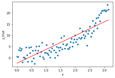
\[\hat{y} = \hat{\beta}_0 + \hat{\beta}_1 x\]

lm = LinearRegression()
lm.fit(df, y)
sns.lineplot(x="x", y=lm.predict(df), 
            color='r', data=df, ax=fig.gca())
fig

The estimated values from the data of the coefficients are \(\hat{\beta}_0\) (the intercept) and \(\hat{\beta}_1\) (the slope w.r.t x1 = x).

lm.intercept_, lm.coef_

(-2.438624719373448, array([6.1438942]))

So we can replace them here in the equation.

\(\hat{\beta}_0\) = -2.44 , \(\hat{\beta}_1\) = 6.14

\[y = -2.44 + 6.14 * x_1\]

The model is rather simplistic, too simple to catch all the fluctuations in the data, it is said to be biased. This results in a systematic made error.

Adding a new feature \(e^x\)

By creating a new feature: \(x_2 = e^x\)

we can still fall back to a linear regression model (linear in its coefficients \(\beta_s\), still expressed as:

\[y = \beta_0 + \beta_1x_1 + \beta_2 x_2 + ... \beta_n x_n + \epsilon_i\]

but this time with \(x_1 = x\) and \(x_2 = e^x\), and based on our data, we have:

\[\hat{y} = \hat{\beta}_0 + \hat{\beta}_1 x + \hat{\beta}_2 e^x\]

We knew already the data was generated by an exponential with some noise around it, so it is no surprise this new model from the same family will better fit the data.

df["expx"] = np.exp(df.x)

lm = LinearRegression()
lm.fit(df, y)
sns.lineplot(x="x", y=lm.predict(df), 
            color='g', data=df, ax=fig.gca())
fig

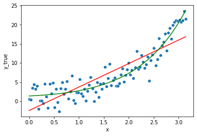
Though if we check the estimated coefficients:

lm.intercept_, lm.coef_

(0.2940994866054796, array([-0.45989402,  1.07636463]))

and replacing them accordingly in the former expression:

\[\hat{y} = -0.51 + 0.455 * x_1 + 0.93 * x_2\] \[\Leftrightarrow \hat{y} = -0.51 + 0.455 * x + 0.93* e^x\]

We can see it leans on a non-null x1 (=x), while the model wasn’t expressed directly linearly w.r.t to variations on x.

Would we have more data, the estimated \(\hat{\beta}_1\) coefficient for x1, should get closer to 0.

What if we put many more features ?

We know already those features were not part of the data generation process. But still.

df["sinx"] = np.sin(df.x)
df["cosx2"] = np.cos(df.x**2)
df["cosx_expx"] = np.cos(df.x) * np.exp(df.x)
df["sin2x"] = np.sin(df.x**2)
df["x3"] = np.sin(df.x**3)
df["sin3x"] = np.sin(df.x)**3
df["xexpx"] = df.x * np.exp(df.x)
df["x*cosx"] = np.cos(df.x)* df.x
df["x4"] =  df.x**4
df["x4*cosx"] = np.cos(df.x)* df.x**4

df.head()

	x	expx	sinx	cosx2	cosx_expx	sin2x	x3	sin3x	xexpx	x*cosx	x4	x4*cosx
0	0.000000	1.000000	0.000000	1.000000	1.000000	0.000000	0.000000	0.000000	0.000000	0.000000	0.000000	0.000000
1	0.031733	1.032242	0.031728	0.999999	1.031722	0.001007	0.000032	0.000032	0.032756	0.031717	0.000001	0.000001
2	0.063467	1.065524	0.063424	0.999992	1.063379	0.004028	0.000256	0.000255	0.067625	0.063339	0.000016	0.000016
3	0.095200	1.099879	0.095056	0.999959	1.094898	0.009063	0.000863	0.000859	0.104708	0.094769	0.000082	0.000082
4	0.126933	1.135341	0.126592	0.999870	1.126207	0.016111	0.002045	0.002029	0.144112	0.125912	0.000260	0.000258

lm = LinearRegression()
lm.fit(df, y)
sns.lineplot(x="x", y=lm.predict(df), 
            color='purple', data=df, ax=fig.gca())
fig

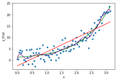
We see the model “seems” to fit even better the data. But does it ?
Actually as you made your model more complex, this model is less biased (the systematic error is greatly reduced) but to a point where the model know even fits the noise, which should actually be an irreducible error on its own.
The model will not likely generalise well to unseen data as we will see later.

Overfitting occurs when a model is too complex, for a linear regression, it tends to be such when it has too many parameters compared to the number of data points (e.g. fitting a n-degree polynomial to n-1 points).

Problem 2: broken regression using a decision tree Regressor

The data

Let’s generate some new data and target for this regression problem.

df = pd.DataFrame(dict(
        x=np.concatenate(
            (np.linspace(0, 5, 10),
             np.linspace(10, 15, 10),
             np.linspace(30, 39, 20),
             np.linspace(40, 49, 10),
             np.linspace(50, 70, 10)))
))

# generate some data for the example
y1 = np.random.uniform(10,12,10)
y2 = np.random.uniform(20,25,10)
y3 = np.random.uniform(0,5,20)
y4 = np.random.uniform(30,32,10)
y5 = np.random.uniform(13,17,10)
y = np.concatenate((y1,y2,y3,y4,y5))

And plot te data:

fig = plt.Figure()
sns.scatterplot(x="x", y=y, data=df, ax=fig.gca())
fig

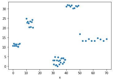
Framework

What is a decision tree ?

Decision Trees (DTs) are a non-parametric supervised learning method used for classification and regression.

\(\Leftrightarrow\) a sequence of non-explicitly programmed if-else condition you will see what i mean in a bit

**Note that the sklearn module does not support missing values. **

Simple to understand and to interpret (not like a ANN). Trees can be visualised
Requires little data preparation (no need to prepare dummy variables for categorical variables)
handle both categorical and numerical variables.

Some disadvantages are:

can create over-complex low biased schemas, but that does not generalize well => it tends to captures the noise of the data, rather than catching the overall trend.
might be unstable to small variations in the data.

Fitted models

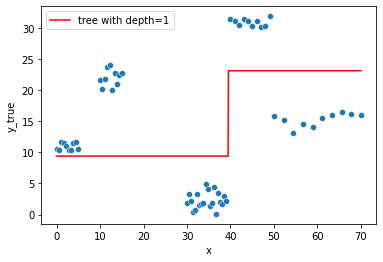
Let’s create 2 decision tree models with max_depth=1 and max_depth=2 respectively:

# a tree with depth = 1
tree = DecisionTreeRegressor(max_depth=1)
tree.fit(df, y)

# another tree with depth = 2
tree2 = DecisionTreeRegressor(max_depth=2)
tree2.fit(df, y)

For the first Decision Tree model:

sns.lineplot(x="x", y=tree.predict(df), 
            color='r', data=df, ax=fig.gca(),
            label="tree with depth=1").set_ylabel("y_true")
fig

And the second one:

sns.lineplot(x="x", y=tree2.predict(df), 
            color='g', data=df, ax=fig.gca(),
            label="tree with depth=2").set_ylabel("y_true")
fig

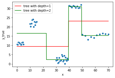
We have a “piecewise” broken prediction line in both cases. (don’t be confused, matplotlib still tries to connect the points when using plt.plot, hence the apparent negative slope between 15 and 30, on the green line, does not exist in practice).

Introspect the model

Let’s introspect the first tree.

def create_and_show_tree(data, y, estimator, ax=None):
    if not ax:
        fig, ax = plt.subplots(1, 1, figsize=(estimator.max_depth*5,5))
    estimator.fit(data, y)
    _ = plot_tree(estimator, ax=ax, fontsize=12)
    return estimator

create_and_show_tree(df, y, DecisionTreeRegressor(max_depth=1) )

DecisionTreeRegressor(max_depth=1)

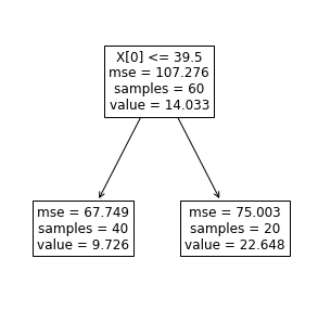
the MSE came back ! MSE = mean of the squared errors.

But which “errors” are we talking about ?

On the root node, the errors on the training dataset from an “hypothetical” very simple model where: \(\hat{y} = mean(y)_{training_data}\)

this is actually the definition of the variance of the target y (<=> the variance is the average of the squared differences from the mean).

Let’s define the MSE in Python:

mse = lambda y, y_pred: np.mean((y - y_pred)**2)

Let’s compute the first MSE before split.

MSE = mse(y, np.mean(y))
MSE

107.27602396460631

ax = sns.scatterplot(x="x", y=y, data=df)
ax.axhline(y=np.mean(y), color='r', label=f"MSE={MSE:0.1f}")
for ix,iy in zip(df.x,y):
    plt.arrow(ix, iy, 0, -(iy-np.mean(y)), head_width=0.10, color="green", length_includes_head=True)
plt.legend()
plt.tight_layout()

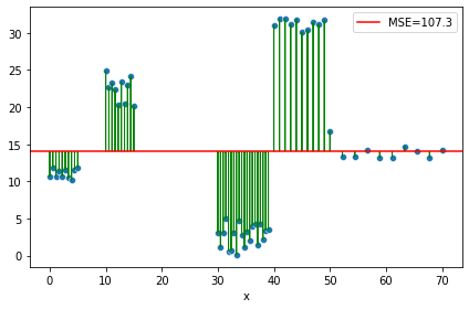
We seek out an overall decrease in this variance by splitting the dataset on a given attribute, to output different, closer, “groupwise”/piecewise \(\hat{y}\).

When there are multiple attributes to choose to split the dataset on, the one producing the highest variance reduction is picked.

The decision tree algorithm would then assess where (the rule) it could partition the data into two to achieve the greatest reduction in overall MSE.
We have only one attribute, let’s choose it, and scroll on the whole range of the axis x.

This is the rule for splitting, on attribute \(x1 = x\):

tresh = tree.tree_.threshold[0]
tresh

39.5

fig, axes = plt.subplots(1,2, figsize=(11,5))
sns.scatterplot(x="x", y=y, data=df, ax=axes[0])
sns.lineplot(x="x", y=tree.predict(df.loc[df.x < tresh]), 
            color='r', data=df.loc[df.x < tresh], ax=axes[0], 
            label=f"MSE={mse_child1:0.1f}").set_ylabel("y_true")
sns.lineplot(x="x", y=tree.predict(df.loc[df.x >= tresh]), 
            color='r', data=df.loc[df.x >= tresh], ax=axes[0], 
            label=f"MSE={mse_child2:0.1f}").set_ylabel("y_true")
for ix,iy in zip(df.x,y):
    ix = np.array([ix])[:,np.newaxis]
    axes[0].arrow(ix, iy, 0, -(iy-float(tree.predict(ix))), head_width=0.10, color="green", length_includes_head=True)
create_and_show_tree(df, y, DecisionTreeRegressor(max_depth=1), axes[1])

DecisionTreeRegressor(max_depth=1)

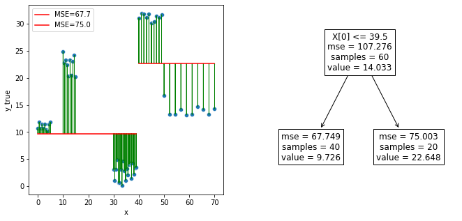
Let’s recompute the overall MSE.

mse(y, tree.predict(df))

70.16706950247945

We can even compute variance in y within each group formed by the split, which can also be seen as the local MSE between \(y\) and \(\hat{y}\) within each child node.

Let’s do the same within each child node

combine_x_y = pd.concat([df, pd.Series(y).to_frame('y')], axis=1)
combine_x_y_child1 = combine_x_y.loc[combine_x_y.x < tresh]
combine_x_y_child2 = combine_x_y.loc[combine_x_y.x >= tresh]

mse_child1 = mse(combine_x_y_child1.y, 
                 tree.predict(combine_x_y_child1[['x']]))
mse_child2 = mse(combine_x_y_child2.y, 
                 tree.predict(combine_x_y_child2[['x']]))
mse_child1, mse_child2

(67.74905504225981, 75.00309842291871)

We can see the former plot produced by scikit gives the same results.

Onwards to hyperparameters

We can set maxdepth before training anything. This is called an hyperparameter.

The hyperparemeter is set prior to the learning process and may influence it.

Here, from maxdepth=2, here is the built tree from the training data:

create_and_show_tree(df, y, DecisionTreeRegressor(max_depth=2))

DecisionTreeRegressor(max_depth=2)

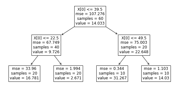
Adding one feature and setting maxdepth=3, here is the tree we got:

df["exp_x"] = np.exp(df.x)
create_and_show_tree(df, y, DecisionTreeRegressor(max_depth=3))

DecisionTreeRegressor(max_depth=3)

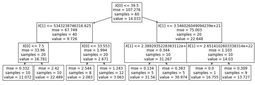
Setting 2 other hyperparameters to some values we may get different trees on the same data used for training (actually the whole data we have here):

create_and_show_tree(df, y, DecisionTreeRegressor(
                max_features=1, max_depth=3, min_samples_leaf=15))

DecisionTreeRegressor(max_depth=3, max_features=1, min_samples_leaf=15)

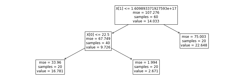
The tree can even become asymetrical as you can see.

Changing again some hyperparameter values:

create_and_show_tree(df, y, DecisionTreeRegressor(
     max_depth=3, min_samples_leaf=10))

DecisionTreeRegressor(max_depth=3, min_samples_leaf=10)

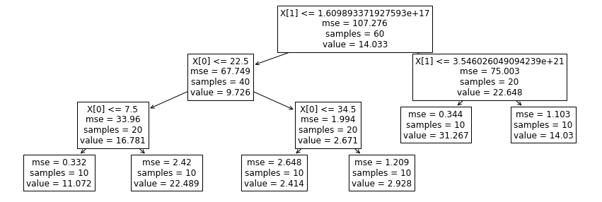
What about creating a tree with a very huge max depth ?

df.drop("exp_x", axis=1, inplace=True)

tree = DecisionTreeRegressor(min_samples_leaf=1)
tree.fit(df, y)

DecisionTreeRegressor()

fig = plt.Figure()
sns.scatterplot(x="x", y=y, data=df, ax=fig.gca())
to_predict = np.linspace(0, 100, 1000)
sns.lineplot(x=to_predict, 
             y=tree.predict(to_predict[:, np.newaxis]),
             color='r', ax=fig.gca(),
             label=f"tree with depth={tree.tree_.max_depth}"
            ).set_ylabel("y_true")
fig

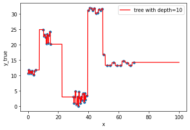
We have 1 sample per leave after leaving the tree grow till only max_depth=9

tree.tree_.n_leaves, tree.tree_.node_count, tree.tree_.max_depth

(60, 119, 10)

tresholds = [ x for x in tree.tree_.threshold if x!=-2 ]

ax = fig.gca()
for line in tresholds:
    ax.axvline(line, color='g')
fig

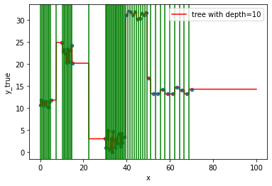
This is what we call overfitting, the noise in the data has been completely captured, not the overall trend…

Random Forest Regression

Framework

It is an ensemble model i.e. multiple models are used to predict an outcome.

It fits multiple decision trees on various sub-samples of the dataset and uses averaging (mean/average prediction of the individual trees) to control over-fitting.

fitted model

rf = RandomForestRegressor(n_estimators=4, max_depth=1)

n_estimators is the number of trees you want to create.

rf.fit(df, y)

RandomForestRegressor(max_depth=1, n_estimators=4)

Let’s check at the estimators = the models this ensemble model is constituted of.

rf.estimators_

[DecisionTreeRegressor(max_depth=1, max_features='auto', random_state=1936295692),
 DecisionTreeRegressor(max_depth=1, max_features='auto', random_state=1302672136),
 DecisionTreeRegressor(max_depth=1, max_features='auto', random_state=1367348600),
 DecisionTreeRegressor(max_depth=1, max_features='auto', random_state=513403266)]

Oh ! Those are Decision Trees !

fig, axes = plt.subplots(1, len(rf.estimators_), figsize=(20, 5))
for i, tree in enumerate(rf.estimators_):
    plot_tree(tree, ax=axes[i], fontsize=12)

Of course i constrained all the trees to have max_depth=1 for visualization purposes but you could have left them growing.
We will see in the next section what would such approach imply in terms of bias and variance.

Predictions

For 1 point, all the trees are going to output a prediction.

Then, the default behavior is to average all the predictions to give the final output.

all_preds = []
for tree in rf.estimators_:
    all_preds.append(tree.predict([[21]]))
all_preds

[array([11.72028749]),
 array([9.28916836]),
 array([9.78519446]),
 array([11.58026019])]

np.mean(all_preds)

10.593727623938157

Comparing to the output directly using the sklearn estimator API.

rf.predict([[21]])

array([10.59372762])

Would you have choosen to leave each constituent trees fully grow, taken individually, they would all be overffiting to the data (this can be reduced by the bagging and feature sampling).
But as the final prediction is made from averaging all of the decision tree predictions, it will naturally reduce the ensemble model variance hence the overffiting itself.

Gradient Boosting Regressor

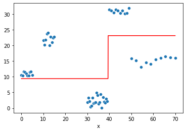
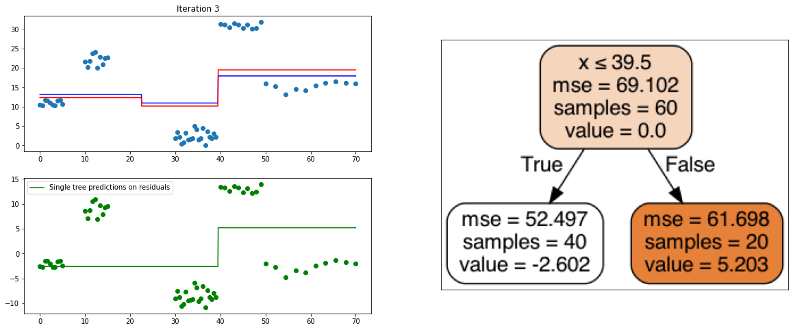
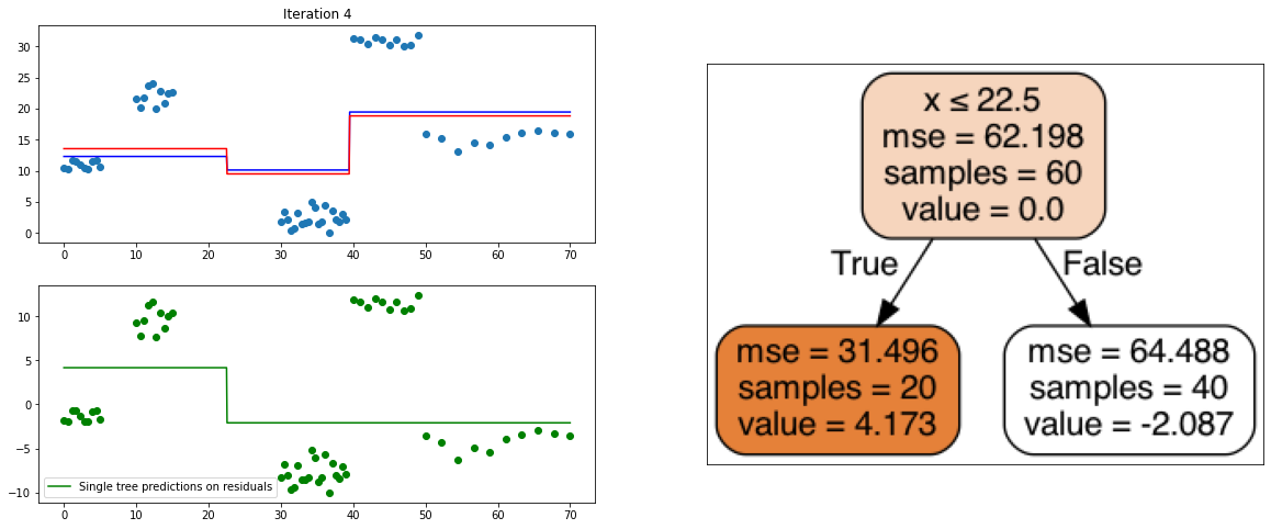
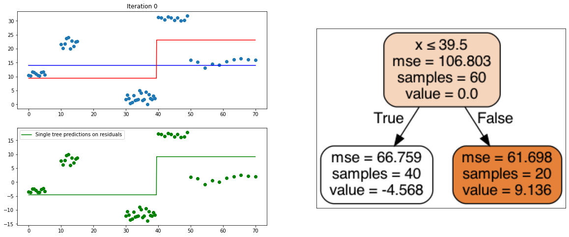
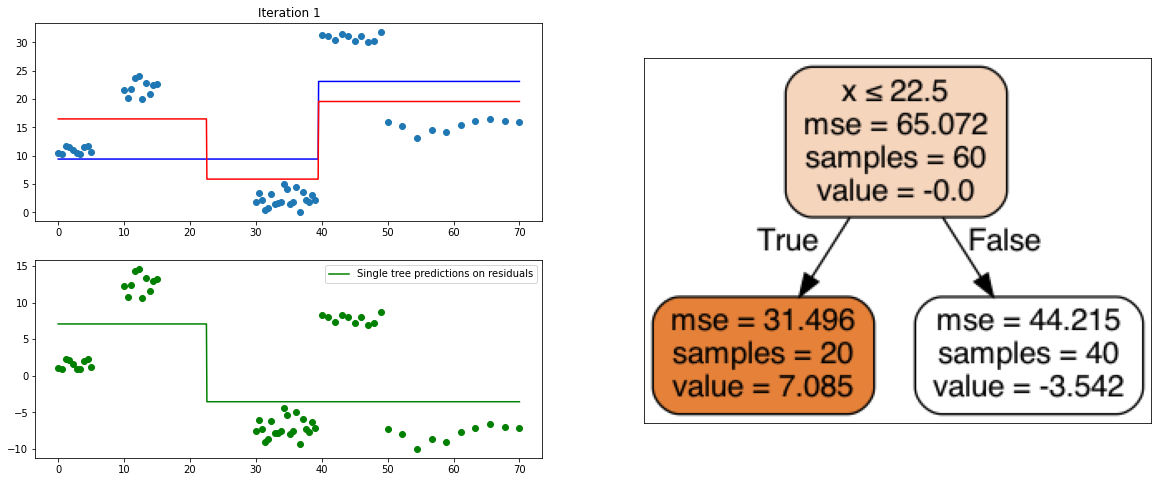
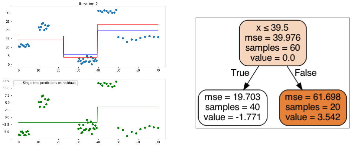
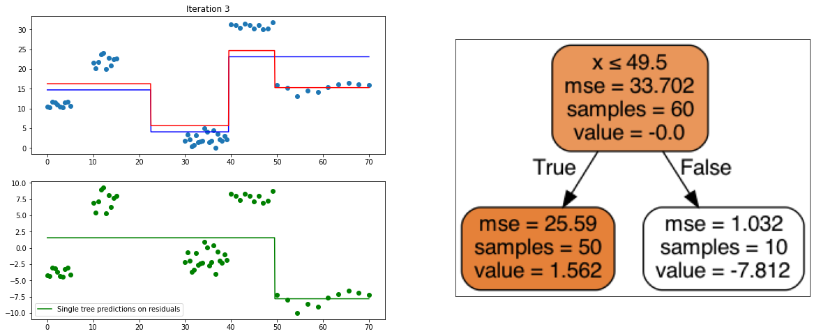
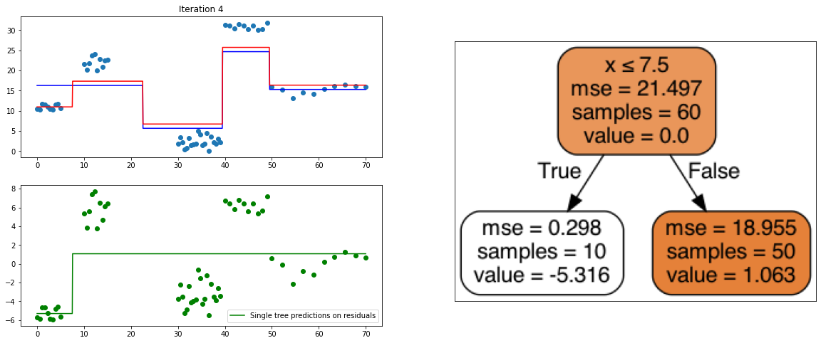
It also is a ensemble model, Regression trees (prefered constituent model) are built sequentially. Hence, at each step, a regression tree model is fit on the residuals (negative gradient) left from the previous one, so to compensate its weaknesses.

It will then be added to the ensemble at prediction stage.

fig = plt.Figure()
sns.scatterplot(x="x", y=y, data=df, ax=fig.gca())
fig

tree = DecisionTreeRegressor(max_depth=1)
tree.fit(df,y)

sns.lineplot(x=df.x, 
             y=tree.predict(df), color='r', ax=fig.gca())
fig

def create_tree_graph(model, df):
    from six import StringIO
    import pydotplus
    from sklearn.tree import export_graphviz
    
    dot_data = StringIO()
    export_graphviz(model, out_file=dot_data,  
                    filled=True, rounded=True,
                    special_characters=True, 
                    feature_names=df.columns)
    graph = pydotplus.graph_from_dot_data(dot_data.getvalue())  
    
    return graph.create_png()

def create_gradient_descent_demo(df, y, lr=0.3, iterations=10):
    # to avoid matplotlib creating a false "slope" to connect points further away 
    x = np.linspace(df.x.min(), df.x.max(), 1000)
    
    xi, yi = df[["x"]].copy(), y.copy()

    # Initialize predictions with average
    predf = np.ones(len(yi)) * np.mean(yi)
    
    # same predictions on lot of x points
    predf_x = np.ones(len(x)) * np.mean(yi)
    
    
    # Compute residuals
    ei = y.reshape(-1,) - predf
    
    # Iterate according to the number of iterations chosen
    for i in range(iterations):
        
        # creating the plot
        # Every iteration, plot the prediction vs the actual data
        # Create 2x2 sub plots
        fig, axes = plt.subplots(figsize=(20,8))
        gs = gridspec.GridSpec(2, 2)
        plt.subplot(gs[0, 0])
        plt.title("Iteration " + str(i))
        
        plt.scatter(xi, yi)
        plt.plot(x, predf_x, c='b', label="Previous predictions")

        # Fit the a stump (max_depth = 1) on xi, ei
        tree = DecisionTreeRegressor(max_depth=1).fit(xi, ei)
        
        # Final predictions
        pred_new = predf + lr * tree.predict(xi)
        
        # Final predictions on lot of x points
        pred_new_x = predf_x + lr * tree.predict(x[:, np.newaxis]) 
        # plotting
        plt.plot(x, pred_new_x, c='r', label='Overall predictions (learning rate)')
        
        # previous residuals, on which the tree is fit
        plt.subplot(gs[1, 0])
        plt.scatter(df.x, ei,  c='g')
        plt.plot(x, tree.predict(x[:, np.newaxis]), c='g', label='Single tree predictions on residuals')
        plt.legend()
        
        # Compute the new residuals,
        ei = y.reshape(-1,) - pred_new
        plt.legend()
        
        axis = plt.subplot(gs[:, 1])
        plt.imshow(imageio.imread(create_tree_graph(tree, df)))
        axis.xaxis.set_visible(False)  # hide the x axis
        axis.yaxis.set_visible(False)  # hide the y axis


        #plt.savefig('bonus_ressources_gradient_boosting/iterations/imgs_iteration{}.png'.format(str(i).zfill(2)))
        plt.show()
        # update
        predf = pred_new
        predf_x = pred_new_x

create_gradient_descent_demo(df, y, lr=0.3, iterations=5)

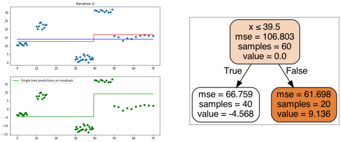
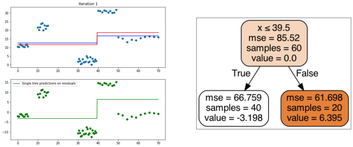
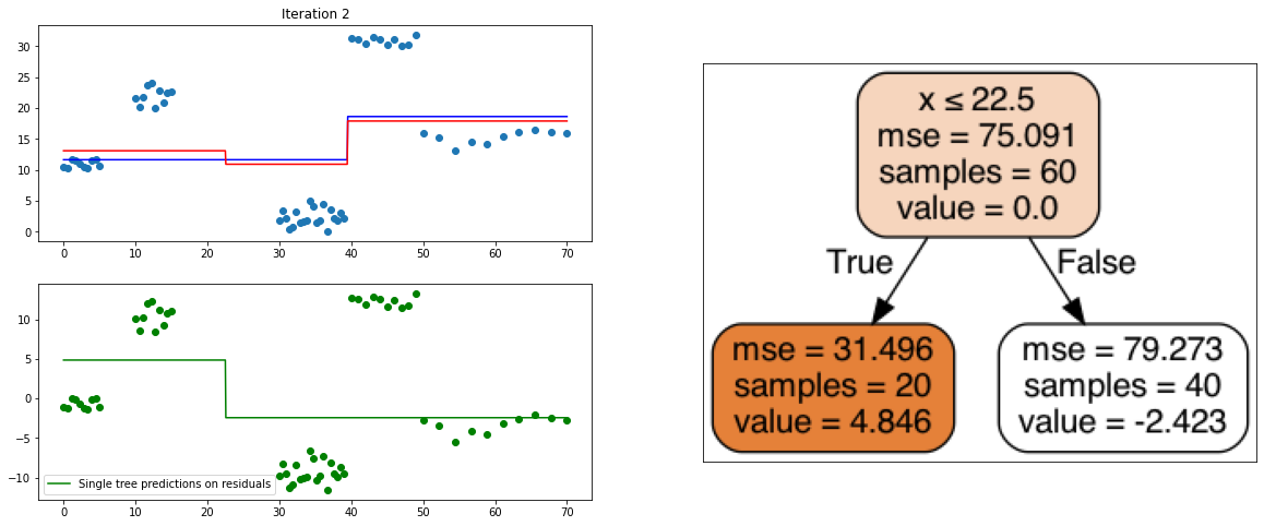
create_gradient_descent_demo(df, y, lr=1, iterations=5)

KNN Regressor

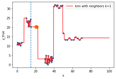
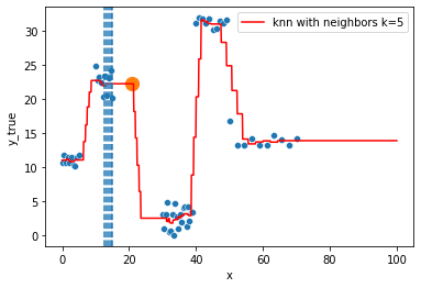
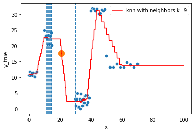
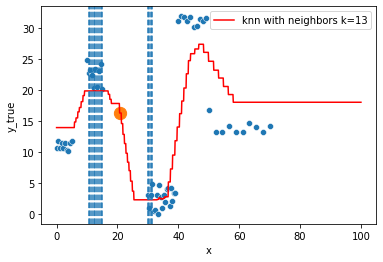
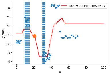
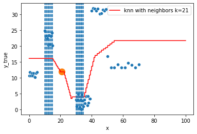
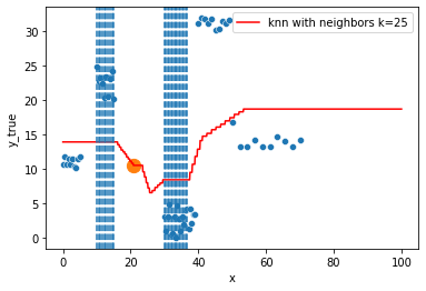
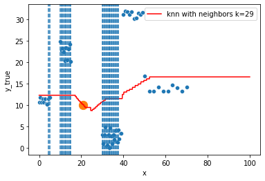
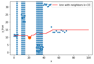
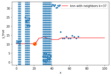
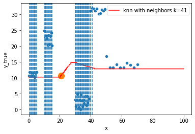
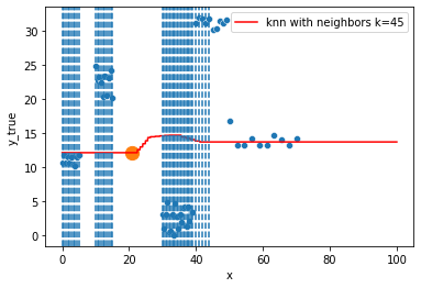
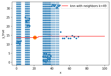
The target is predicted by local interpolation of the targets associated to the nearest neighbors (k closest training examples in the feature space) in the training set.

for k in range(1, 50, 4):
    fig = plt.figure()
    sns.scatterplot(x="x", y=y, data=df, ax=fig.gca())
    to_predict = np.linspace(0, 100, 1000)

    knn = KNeighborsRegressor(n_neighbors=k)
    knn.fit(df, y)
    sns.lineplot(x=to_predict, 
                 y=knn.predict(to_predict[:, np.newaxis]),
                 color='r', ax=fig.gca(),
                 label=f"knn with neighbors k={knn.n_neighbors}"
                ).set_ylabel("y_true")
    ax = fig.gca()
    
    xi = np.array([21])
    # select k nearest neighbors x indexes
    indexes = abs(df.x  - xi).sort_values().head(k).index
    ax.scatter(x=xi, y=knn.predict(xi[:, np.newaxis]),
               s=150)
    
    neighbors_x = df.loc[indexes, "x"]
    for neighbor in neighbors_x:
        ax.axvline(neighbor, linestyle="--")

    plt.show()

Hyperparameter tuning

We have been looking at some models already, some had hyperparameters. Which “best” values should we pick for them to get the best achieving model ?

A matter of bias/variance trade-off

Let’s first go back to the data and check how are performing some KNN and Decision Tree models

# generate some data for the example
y1 = np.random.uniform(10,15,10)
y2 = np.random.uniform(20,30,10)
y3 = np.random.uniform(0,5,20)
y4 = np.random.uniform(30,40,10)
y5 = np.random.uniform(13,17,10)
y = np.concatenate((y1,y2,y3,y4,y5))
fig = plt.Figure()
sns.scatterplot(x="x", y=y, data=df, ax=fig.gca())
fig

# a tree with depth = 1
tree = DecisionTreeRegressor(max_depth=1)
tree.fit(df, y)
# another tree with depth = 3
tree2 = DecisionTreeRegressor(max_depth=3)
tree2.fit(df, y)
# another tree with depth = 8
tree3 = DecisionTreeRegressor(max_depth=8)
tree3.fit(df, y)

fig, axes = plt.subplots(1, 3, figsize=(14,5))
for ax in axes:
    sns.scatterplot(x="x", y=y, data=df, ax=ax)

# to avoid matplotlib creating a false "slope" to connect points further away 
x = np.linspace(df.x.min(), df.x.max(), 1000)
sns.lineplot(x=x, y=tree.predict(x[:, np.newaxis]), 
            color='r', ax = axes[0],
            label="tree with depth=1").set_ylabel("y_true")
sns.lineplot(x=x, y=tree2.predict(x[:, np.newaxis]), 
            color='b', ax = axes[1],
            label="tree with depth=3").set_ylabel("y_true")
sns.lineplot(x=x, y=tree3.predict(x[:, np.newaxis]),
            color='g', ax = axes[2],
            label="tree with depth=8").set_ylabel("y_true")

# the data
data = pd.DataFrame(dict(
    x = np.linspace(0, np.pi, 100),
    y_true = np.random.normal(np.exp(x), scale=2.0)))
df, y = data.drop("y_true", axis=1), data.y_true

# the figure and axes
fig, axes = plt.subplots(1, 3, figsize=(14,5))
# plot the scatter plots on each ax
for ax in axes:
    sns.scatterplot(x="x", y=y, data=df, ax=ax)

estimators = []
ks = [1, 10, 80]

# for index i of axes, number k of neighbors
for k in ks:
    # fit a KNN model with k neighbors
    knn = KNeighborsRegressor(n_neighbors=k)
    knn.fit(df, y)
    # save the knn model
    estimators.append(knn)
    
for i, knn in enumerate(estimators):
    to_predict = np.linspace(df.x.min(), df.x.max(), 1000)
    sns.lineplot(x=to_predict, 
                 y=knn.predict(to_predict[:, np.newaxis]),
                 color='r', ax = axes[i],
                 label=f"knn with neighbors k={knn.n_neighbors}"
                ).set_ylabel("y_true")

alpha = 1
# point to predict
prediction_point = np.array([2.6])
for i, knn in enumerate(estimators):
    # find the closest neighbor in the feature space used for the predictions
    # and locate them by plotting them
    indexes = abs(df.x  - prediction_point).sort_values().head(knn.n_neighbors).index
    neighbors_x = df.loc[indexes, "x"]
    
    for neighbor in neighbors_x:
        axes[i].axvline(neighbor, linestyle="--", alpha=alpha)
    alpha -= 0.3
    # plot the prediction using knn estimator 
    axes[i].scatter(x=prediction_point,
                    y=knn.predict(prediction_point[:, np.newaxis]),
                    s=200, 
                    c='orange')

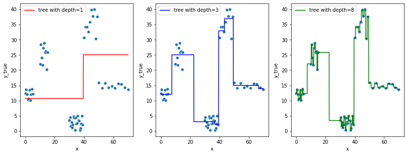
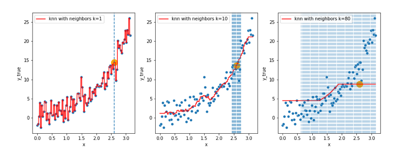
In the first set of figures (decision trees), does the model showed on the right really look better than the one on the left ? 🤔
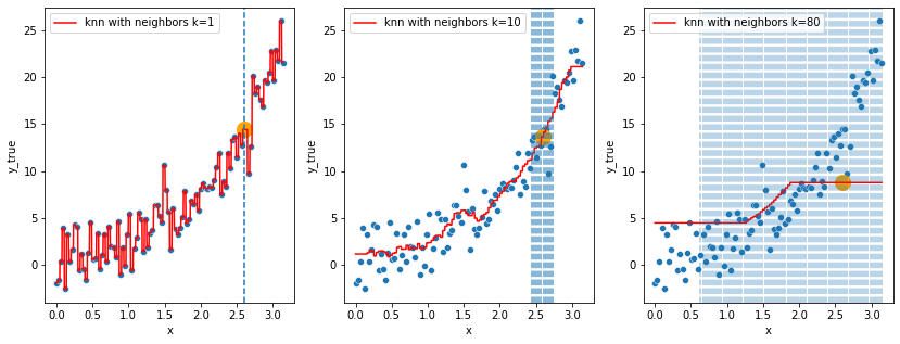
In the second set of figures (knn), does the model on the left really look better than the one on the right ? 🤔

In both of these 2 cases, the models got so complex that they actually started learning the noise in the training data, this is a great example where the bias (systematic error) is low, but the generalization of the model is not guaranteed, i.e. the model variance is very high, we call this phenomenon overfitting.

In the other way around (left side in figure 1, right side in figure 2), the models showed the actual inverse, that is, underfitting (“immutable” model due to its simplicity built from exagerated reductive assumptions)

To assess overfitting issues, one can use cross-validation techniques !

X_train, X_test, y_train, y_test = train_test_split(df, y, test_size=0.2) 

X_train.shape, X_test.shape, y_train.shape, y_test.shape

((48, 1), (12, 1), (48,), (12,))

By splitting the dataset into training and test sets, you can validate whether your model will generalize well to unseen data. We fit the model on the training set, we evaluate on the train and above all test set.

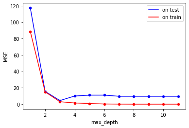
Hence if the model has started learning the noise in the training data, you should expect that:

\[MSPE(training_{data}) < MSPE(test_{data})\]

How to make our model simpler, that is introduce more bias to lower the variance, when we have no idea of which of the branch, coefficients, or other model construct should be discarded ? We can act on regularization techniques.

In most ML algorithms, regularization techniques are introduced as hyperparameters you set to constrain your model into not trying to learn overly-complex (and often misleading) patterns in the data.

You’ve actually crossed some multiple times: have a look at the max_depth and min_samples_leaf or min_samples_split for example ! What do you think we should prune a tree for ?

Tuning hyperparameters (or data processing steps)

Ok so, we know we could fit a model on a train set and later compute a MSE on both the train, and test set to assess whether an overfit would have occured. And overfitting can be seen on the right models. We know that we can act on some hyperparameters like max_depth to regularize such an overfit, and we wish to lower down the MSE(test set) as much as we could get it (as MSE encapsulates both bias and variance term, we would be guaranted the model perform well in practice and generalize well either)!

Cross-validation is the simplest method for estimating the expected prediction error i.e. the expected extra-sample error for when we fit a model to a training set and evaluate its predictions on unseen data.

For an hyperparametrized model such as the DecisionTree, that would actually be quite nice if we could find the best max_depth to achieve the best MSE on test set.

One again, of course we are not going to control which max_depth value to finally pick based on the MSE of the training set: that would lead exactly to the very first situation where we shaped our mind, our representation of our data and our modelisation out of it to solely satisfy ourself on what we know, rather than what we don’t yet loosing all the predictive ability of our model, and getting back to the overfitting/generalization issue.

So we will try multiple values of max_depth and later check the MSE on the test set, in a bid to reduce it.

sns.lineplot(x="max_depth", y="MSE(test)", color='b',
                data= pd.DataFrame(MSE_test.items(), columns=["max_depth", "MSE(test)"]), label="on test")
sns.lineplot(x="max_depth", y="MSE(train)", color='r',
                data= pd.DataFrame(MSE_train.items(), columns=["max_depth", "MSE(train)"]), label="on train")
sns.scatterplot(x="max_depth", y="MSE(test)", color='b',
                data= pd.DataFrame(MSE_test.items(), columns=["max_depth", "MSE(test)"]))
sns.scatterplot(x="max_depth", y="MSE(train)", color='r',
                data= pd.DataFrame(MSE_train.items(), columns=["max_depth", "MSE(train)"])).set_ylabel("MSE")

Text(0, 0.5, 'MSE')

Changing `min_samples_leaf` AND `max_depth`

using a simple loop ?

max_depth_range = range(1, 10)
min_samples_leafs_range = range(1, 10,1)

for i in max_depth_range:
    for j in min_samples_leafs_range:
        pass

better: onwards to GridSearch

param_grid={
    "max_depth" : np.arange(1, 10, 1),
    "min_samples_split": np.arange(2, 20, 3),
}

grid = GridSearchCV(
    estimator=DecisionTreeRegressor(),
    param_grid=param_grid,
    scoring="neg_mean_squared_error",
    cv=KFold(5, shuffle=True)
)

grid.fit(df, y)

GridSearchCV(cv=KFold(n_splits=5, random_state=None, shuffle=True),
             estimator=DecisionTreeRegressor(),
             param_grid={'max_depth': array([1, 2, 3, 4, 5, 6, 7, 8, 9]),
                         'min_samples_split': array([ 2,  5,  8, 11, 14, 17])},
             scoring='neg_mean_squared_error')

grid.best_estimator_

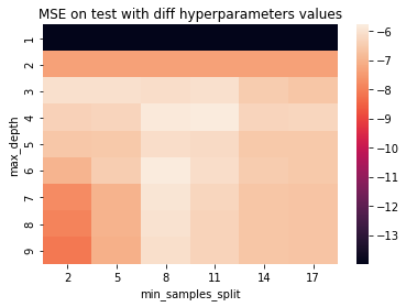
DecisionTreeRegressor(max_depth=6, min_samples_split=8)

df_grid = pd.DataFrame(grid.cv_results_)
params = df_grid.params.apply(pd.Series)
df_grid = pd.concat([params, df_grid], axis=1)

pivot = df_grid.pivot_table(index='max_depth', columns='min_samples_split', values="mean_test_score")

ax = sns.heatmap(pivot)
ax.set_title("MSE on test with diff hyperparameters values")

Text(0.5, 1.0, 'MSE on test with diff hyperparameters values')

Need for a validation set

But if you were to tune hyperparams or data preparation steps while checking variations of MSE on test towards a minimization of it, well, we would still somehow use a metric, a quantitative measure we shouldn’t be aware of, as it is supposed to be the mean squared errors of the model on unseen data.
To give another example: it is as if you had to forecast whether or not to buy vegetables while not having access to the inside of the fridge. If you can weight the fridge itself, you might not know how many vegetables are left among all the food, but at least you have a taste of how likely the fridge is empty, considering the vegetables are the heaviest, hence you modify your behavior respectively.

This has a name: it is called data leakage.

You would have to actually split the whole data in 3 sets: train, validation and test, so to keep at least one set of data only for estimating the expected prediction error of the final model.
You set a max_depth (and/or other hyperparameters) prior to training the model, you train the model on the training set, you monitor the MSE on the validation set, you update max_depth to a new value, and so on. Once you have found a satisfying minimum of the MSE on the validation set, you can retrain on the whole available data (train+validation) and finally evaluate the final model using the hold-out test set.

K-Fold cross validation

Splitting data again and again in an attempt to put Chinese walls in your ML workflow, lead to another issue: what if you don’t have much data? it is likely your MSE(test) on a few dozen points could be overly optimistic, what if by chance you got the right test points to have a sweet MSE that suit your needs for a certain model ?

K-Fold cross validation is an attempt to use every data points at least in the testing part.
It is still cross-validation, but this time you split your dataset in K aproximately equally sized folds.
Then you train the model on K-1 folds and test it on the remaining one. You do it K times (each time tested for each remaining test fold). Yes, you end up with K number of MSE(test-fold).

On a train-test design, the average of the MSE is still a good estimate for the expected prediction error of the model.
On a train-test-validation one, you still have more confidence that no data points were left while computing the MSE “on the test”.

Let’s do a k-fold cross validation on a data generated from a sine function with some noise following gaussian distribution.

cross_val_score(LinearRegression(), x, y, scoring="r2")

array([-0.95596911, -2.89048347,  0.18178379, -5.47694298, -2.31706554])

scoring takes a scoring parameter (greater is better), hence is used the R2 is an appropriate choice, we could have taken the negation of the MSE too.

- cross_val_score(LinearRegression(), x2, y, scoring="neg_mean_squared_error")

array([0.3279406 , 0.45555535, 0.25739018, 1.03002024, 1.27365498])

5 folds
5 model training
5 test sets
5 MSE

Wow ? difference are so important from one test set to another ! why is so ? When the MSE is high, the R2 is low, sometimes negative ? worse than a simple dummy model (H0 hypthesis) using the average. Why is so ?

folding = KFold(5)

folding.split(x2, y)

<generator object _BaseKFold.split at 0x12b2c5430>

Wow ! a generator object !

generator = folding.split(x2, y)



```python
def cross_val_visualize(X, y, cv=5, shuffle=False):
    new_fig, axes =  plt.subplots(figsize=(cv*3, 3), ncols=cv, sharey=True)
    regressions, MSE = [], []
    folds = KFold(cv, shuffle=shuffle).split(X, y)
    
    for i_, (train_indices, test_indices) in enumerate(folds):
        # train on each 4 folds subset
        lm = LinearRegression()
        lm.fit( X[train_indices], y[train_indices])
        # predict on each test fold
        y_pred = lm.predict(X[test_indices])
        # compute MSE for those test fold
        mse = mean_squared_error(lm.predict(X[test_indices]), y[test_indices])
        # plot the training points, test points, and the fit for the fold
        axes[i_].scatter( X[train_indices], y[train_indices], color='r')
        axes[i_].scatter( X[test_indices], y[test_indices], color='g')
        axes[i_].plot( X, lm.predict(X), color='black' )
        # save the results | save the models
        MSE.append(mse); regressions.append(lm)
    return MSE

Fitting on some random splits in the data, the MSE among each split is more homogeneous.

cross_val_visualize(x2, y)

[0.32794060000061515,
45555535076735226,
2573901788986118,
0300202445239781,
273654982470511]

cross_val_visualize(x2, y, 3)

[0.24514477688923542, 0.38705639490105015, 0.6231891770127047]

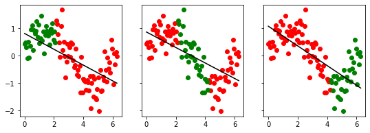
cross_val_visualize(x2, y, shuffle=True)

[0.3711358856524268,
3821283100103246,
5107607283792079,
4372335783422797,
37844005566106576]

Bringing all together

If you followed the previous steps, here is what is going to be the overall scheme of the hyperparameter tuner (you :p)

Splitting the whole dataset in train - test (e.g. of ratios: 0.80 / 0.20 or 0.90/0.10, this depends on your data available).
Leave the test set for a while, it will be used at the end for an estimation of the expected prediction error of the final model.
Select a model (or a set of models) and a set of corresponding hyperparameters. Pick some values for each hyperparameter to try: if you have 2 hyperparameters \(hyper1\) and \(hyper2\), one would do want to try all combinations of the values taken by \((hyper1, hyper2)\) using a hyperparameter grid.
Further split the training set in train and validation, or, if using k-fold cross validation: split into \(k\) different training and validation sets.
If you choose a k-fold, you are going to train the same model & hyperparameter values \(k\) times (one for each partition), and can later compute the mean and std of the MSE results on the k validation sets.
Pick the model which performed the best, using the average MSE.
You can now re-train it on the whole initial training set, the one you had before you further split into train and validation sets.
Evaluate the performance using the held-out test set.

Add-ons

Extract decision rules from a decision tree

Hands-on Supervised Learning with Sklearn - regression model examples

Table Of Contents

Table Of Contents

Some regressions on some data

Imports

Problem 1: data modeled using a linear model

The data

Linear regression model

Statistical population model

Fitted model

Framework

Adding a new feature \(e^x\)

What if we put many more features ?

Problem 2: broken regression using a decision tree Regressor

The data

Framework

What is a decision tree ?

Fitted models

Introspect the model

Onwards to hyperparameters

Random Forest Regression

Framework

fitted model

Predictions

Gradient Boosting Regressor

KNN Regressor

Hyperparameter tuning

A matter of bias/variance trade-off

Tuning hyperparameters (or data processing steps)

Changing `min_samples_leaf` AND `max_depth`

using a simple loop ?

better: onwards to GridSearch

Need for a validation set

K-Fold cross validation

Bringing all together

Add-ons

Join Newsletter

Written by Luc

Hands-on Supervised Learning with Sklearn - regression model examples

Table Of Contents

Table Of Contents

Some regressions on some data

Imports

Problem 1: data modeled using a linear model

The data

Linear regression model

Statistical population model

Fitted model

Framework

Adding a new feature \(e^x\)

What if we put many more features ?

Problem 2: broken regression using a decision tree Regressor

The data

Framework

What is a decision tree ?

Fitted models

Introspect the model

Onwards to hyperparameters

Random Forest Regression

Framework

fitted model

Predictions

Gradient Boosting Regressor

KNN Regressor

Hyperparameter tuning

A matter of bias/variance trade-off

Tuning hyperparameters (or data processing steps)

Changing min_samples_leaf AND max_depth

using a simple loop ?

better: onwards to GridSearch

Need for a validation set

K-Fold cross validation

Bringing all together

Add-ons

Join Newsletter

Written by Luc

Changing `min_samples_leaf` AND `max_depth`